Exploring the Computational Complexity of Linear Optics and its Implications on the ECT
210 likes | 348 Vues
This paper delves into the computational complexity of linear optics, contrasting classical and quantum computations while addressing the Extended Church-Turing Thesis (ECT). It raises critical questions about the efficiency of quantum algorithms, particularly in relation to Shor’s Theorem and the difficulty of simulating quantum systems using classical approaches. Key results establish relationships between sampling problems, decision problems, and the polynomial hierarchy, arguing for the unique capabilities of quantum computers. The work emphasizes the importance of linear optics in advancing our understanding of quantum computation and complexity.

Exploring the Computational Complexity of Linear Optics and its Implications on the ECT
E N D
Presentation Transcript
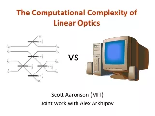
The Computational Complexity of Linear Optics vs Scott Aaronson and Alex Arkhipov MIT
The Extended Church-Turing Thesis (ECT) Everything feasibly computable in the physical world is feasibly computable by a (probabilistic) Turing machine Shor’s Theorem:Quantum Simulation has no efficient classical algorithm, unless Factoringdoes also
So the ECT is false … what more evidence could anyone want? • Building a QC able to factor large numbers is damn hard! After 16 years, no fundamental obstacle has been found (or even seriously proposed), but who knows? • Can’t we “meet the physicists halfway,” and show computational hardness for quantum systems closer to what they actually work with now? • Factoring might be in BPP! At any rate, it’s an extremely “special” problem • Wouldn’t it be great to show that if BPP=BQP, then (say) the polynomial hierarchy collapses?
Today: “A New Attack on the ECT” We define a model of computation based on linear optics: n identical photons traveling through a network of poly(n) mirrors, phase-shifters, etc., then a single measurement of where the photons ended up Crucial point: No entangling interactions between pairs of photons needed! Our model is contained in BQP, but seems unlikely to be BQP-complete. We don’t know if it solves any decision problems that are hard classically. But for sampling and relation problems, the situation is completely different…
Theorem 1. Suppose that for every linear-optics network, the probability distribution over measurement outcomes can be sampled in classical polynomial time. Then P#P=BPPNP (so PH collapses) More generally, let O be any oracle that simulates a linear-optics network A, given a description of A and a random string r. Then So even if linear optics can be simulated in BPPPH, that still collapses PH! (New evidence that QCs have capabilities beyond PH, complementing [A’10],[FU’10]) “OK, but isn’t the real question the hardness of approximate sampling? After all, experiments are noisy, and not even the linear-optics network itself can sample exactly!”
Theorem 2. Suppose two plausible conjectures are true: the permanent of a Gaussian random matrix is (1) #P-hard to approximate, and (2) not too concentrated around 0. Let O be any oracle takes as input a description of a linear-optics network A, a random string r, and 01/, and that samples from a distribution -close to A’s in variation distance. Then In other words: if our conjectures hold, then even simulating noisy linear-optics experiments is classically intractable, unless PH collapses
From Sampling to Relation Problems Let FBPP and FBQP be the classes of relation problems(like finding a Nash equilibrium) that are solvable by classical and quantum computers respectively, in poly(n,1/) time and with success probability 1- Then assuming our conjectures, even FBPP=FBQP would imply P#P=BPPNP Theorem (A., last week):FBPP=FBQPif and only ifSampP=SampBQP. Proof Sketch:SampP=SampBQP FBPP=FBQP is immediate. For the other direction, use Kolmogorov complexity!
Particle Physics In One Slide There are two basic types of particle in the universe… All I can say is, the bosons got the harder job Indeed, [Valiant 2002, Terhal-DiVincenzo 2002] showed that noninteracting fermion systems can be simulated in BPP. But, confirming Avi’s joke, we’ll argue that the analogous problem for bosons (such as photons) is much much harder… BOSONS FERMIONS Their transition amplitudes are given respectively by…
Linear Optics for Dummies We’ll be considering a special kind of quantum computer, which is not based on qubits The basis states have the form |S=|s1,…,sm, where si is the number of photons in the ith “mode” We’ll never create or destroy photons. So if there are n photons, then s1,…,sm are nonnegative integers summing to n For us, m=poly(n) Initial state: |I=|1,…,1,0,……,0
You get to apply any mm unitary matrix U If n=1 (i.e., there’s only one photon, in a superposition over the m modes), U acts on that photon in the obvious way In general, there are ways to distribute n identical photons into m modes U induces an MM unitary (U) on the n-photon states as follows: Here US,T is an nn submatrix of U (possibly with repeated rows and columns), obtained by taking si copies of the ith row of U and tj copies of the jth column for all i,j
Example: The “Hong-Ou-Mandel Dip” U Suppose Then Pr[the two photons land in different modes] is Pr[they both land in the first mode] is
Beautiful Alternate Perspective The “state” of our computer, at any time, is a degree-n polynomial over the variables x=(x1,…,xm) (n<<m) Initial state: p(x) := x1xn We can apply any mm unitary transformation U to x, to obtain a new degree-n polynomial Then on “measuring,” we see the monomialwith probability
OK, so why is it hard to sample the distribution over photon numbers classically? Given any matrix ACnn, we can construct an mm unitary U (where m2n) as follows: Suppose we start with |I=|1,…,1,0,…,0 (one photon in each of the first n modes), apply U, and measure. Then the probability of observing |I again is
Claim 1: p is #P-complete to estimate (up to a constant factor) Idea: Valiant proved that the Permanent is #P-complete. Can use a classical reduction to go from a multiplicative approximation of |Per(A)|2 to Per(A) itself. Claim 2: Suppose we had a fast classical algorithm for linear-optics sampling. Then we could estimate p in BPPNP Idea: Let M be our classical sampling algorithm, and let r be its randomness. Use approximate counting to estimate Conclusion: Suppose we had a fast classical algorithm for linear-optics sampling. Then P#P=BPPNP.
As I said before, I find this result unsatisfying, since it only talks about the classical hardness of exactly sampling the distribution over photon numbers What about sampling a distribution that’s 1/poly(n)-close in variation distance? Difficulty:The sampler might adversarially refuse to output the one submatrixwhose permanent we care about! That changes the output distribution by only exp(-n), so we still have an excellent sampler … but we can no longer use it to estimate |Per(A)|2 in BPPNP To get around this difficulty, it seems we need to “smuggle in” the matrix A that we about as a randomsubmatrix of U
Main Result Consider applying a Haar-random mm unitary matrix U, to n photons in m=poly(n) modes: U Distribution DU over photon numbers Main technical lemma used in proof: Let mn6. Then an nn submatrix of an mm Haar unitary matrix is Õ(1/n)-close in variation distance to a matrix of independent Gaussians. Suppose there’s a classical algorithm to sample a distribution -close to DU in poly(n,1/) time. Then for all ,1/poly(n), there’s also a BPPNP algorithm to estimate |Per(X)|2 to within additive error n!, with probability 1- over a Gaussian random matrix
So the question boils down to this: how hard is it to additively estimate |Per(X)|2, with high probability over a Gaussian random matrix We conjecture that it’s #P-hard—in which case, even approximate classical simulation of our linear-optics experiment would imply P#P=BPPNP We can decompose this conjecture into two plausible sub-conjectures: that multiplicatively estimating Per(X) is #P-hard for Gaussian X, and that Per(X) is “not too concentrated around 0”
The Permanent-of-Gaussians Conjecture (PGC) The following problem is #P-hard. Given a matrix XCnn of i.i.d. Gaussian entries, together with 01/ and 01/, output an approximation z such that We can prove #P-hardness if =0 or =0. So what makes the PGC nontrivial is really the combination of average-case with approximation…
The Permanent Anti-Concentration Conjecture (PACC) There exist constants C,D and >0 such that for all n and >0, Empirically true! Also, we can prove it with determinant in place of permanent
Experimental Prospects It seems well within current technology to do our experiment with (say) n=4 photons and m=20 modes (Current record: n=2 photons) Physicists we consulted: “Sounds hard! But not as hard as building a universal QC” If you can scale to n photons and error in variation distance, using “poly(n,1/) experimental effort,” then modulo our complexity conjectures, the ECT is false • What would it take to scale to (say) n=20 photons and m=500 modes? • Reliable single-photon sources (standard laser isn’t good enough!) • Reliable photodetector arrays • Stable apparatus to ensure that w.h.p., all n photons arrive at photodetector arrays at exactly the same time Remark: No point in scaling this experiment much beyond 20 or 30 photons, since then a classical computer can’t even verify the answers!
Open Problems Prove the PGC ($200) and PACC ($100)! Can our linear-optics model solve classically-intractable decision problems? What about problems for which a classical computer can verify the answers? Do BPP=BQP or PromiseBPP=PromiseBQP have interesting structural complexity consequences? • Similar hardness results for other natural quantum systems (besides linear optics)? • Bremner, Jozsa, Shepherd 2010: Another system for which exact classical simulation would collapse PH