Download
1 / 34
340 likes | 368 Vues
Explore the intricate dynamics of market equilibria, focusing on agent preferences, utility functions, exchanges, and equilibrium theories.

E N D
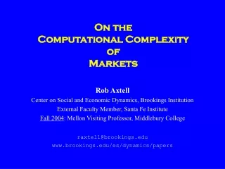
On theComputational ComplexityofMarkets Rob Axtell Center on Social and Economic Dynamics, Brookings Institution External Faculty Member, Santa Fe Institute Fall 2004: Mellon Visiting Professor, Middlebury College raxtell@brookings.edu www.brookings.edu/es/dynamics/papers
Tutorial on General EquilibriumThe Problem Solved by Markets • A population of agents, each with • an endowment of commodities (observable) • a preference ordering over commodity bundles (unobservable) • In general, there exist reallocations of commodities that make agents better off • Prices decentralize the determination of such reallocations
Agent Preferences • Each agent has preferences over states of the world, i.e., for all states, s1 and s2, either: • s1 fs2, • s2 fs1, or • s1 fs2and s2 fs1in which case define s1 ~ s2 • f is a binary relation with properties reflexivity, completeness, transitivity, and continuity
Commodities • There exist Ncommodities (aka goods) in the economy (market) • The commodity space, XRN+, X compact • Agent i’s commoditybundle, xiX • Proposition: For f a binary relation on X, there exists a maximal element, x* X
Agent Utility • Call P the set of all preference orders on X • A preference order, f P, is monotonic if x ≥ y and x ≠ y implies xf y for every x, y in X(more is better) • A utility function for f P is a continuous function U: X R with the property that U(x)>U(y) iff x f y • Theorem: For every fP there exists a utility function, Ui: X R
Distributions and Redistributions • Each agent is a point in (P, X) • Set of agents: A, | A | = A • A distribution (aka allocation), x (x1, x2,..., xA) (X, X,…, X) X • An endowment (aka initial distribution), ex(t=0) • Agent i’s commodity bundle, xi, is individually rational for i if xi fei • A distribution, x, is individually rational if xfe • A redistribution (aka feasible distribution) is a distribution, x, s.t. SiAxi = SiA ei
Exchange and Optimality • An exchange economy (market), is a mapping E: A Xfrom preferences and endowments into individually rational redistributions • A distribution, x, is Paretooptimal (aka efficient) if there exists no redistribution, y, such that y f x
Agent Demands • Commodity prices, p (p1, p2,..., pN) • Agent i’s budget, Bip ei • Agent i’s budget set, bi(p, ei) {xi X | p xi p ei} • Agent i’s demand set, di(p, ei) {xi bi(p, ei) | xi f yi for all yi bi(p, ei)}
Equilibrium • A Walrasian equilibrium of an exchange economy (market) is an individually rational redistribution, x, and prices, p, s.t. xi di(p, ei) for all i A • Call W the set of all Walrasian equilibria
Existence of Exchange Equilibrium(First Welfare Theorem/“Invisible Hand” Theorem) • Aggregate demand: D(p) = SiAdi(p, ei) • Excess demand: Z(p) = SiAdi(p, ei) - SiAei • Proposition: For every exchange economy composed of agents having monotonic preferences there exists a price vector, p*, s.t. Z(p*) = 0, hence a Walrasian equilibrium • First Welfare Theorem: Walrasian equilibria are Pareto optimal
Brouwer Fixed Point Theorem • Theorem: Suppose that R RM is a nonempty, compact, convex set, and that f: R R is a continuous function from R into itself. Then f has a fixed point; that is, there is an x* R s.t. x* = f(x*) • Original proof is non-constructive • Constructive proof through Sperner’s lemma
Motivation for Agents, I:Invisible Hand/First Welfare Theorem • Conventional view (e.g., Stokey and Lucas): • First welfare theorem is formalization of Smithian ‘indivisible hand’ • Economic philosophers/historians of thought (e.g., Nozick): • ‘Invisible hand explanations’ require process • First welfare theorem fails on these grounds • Today, no satisfactory rationalization of Smith’s ideas • Equation of two concepts is half-baked due to centralized character of prices
Motivation for Agents, II:Computation of Walrasian Equilibria • Ostensibly, the job of an ‘auctioneer’ • Scarf algorithm (instantiation of Sperner’s lemma) guarantees convergence • Basis for CGE models • Nasty dependence on the commodity space size • Not credible as a behavioral specification • Prices emerge from the interactions of agents • Top-down/centralized character of such computations vitiates decentralized market interpretations
Motivation for Agents, III:Agent-Based Financial Market Models • Interacting agents who perpetually adapt their behavior to current circumstances • Lux model: • 2 kinds of traders, fundamentalist and chartist • Reproduces empirical features of financial markets (e.g., heavy-tailed returns, volatility clustering, and so on) • LeBaron model: • Traders with spectrum of time horizons • ‘Defection’ to short horizon always welfare-improving • Market of short horizon traders reproduces most empirical features of financial markets
Motivation for Agents, IV:Treat markets as a distributed computation deviceWhat can be computed? • Can markets of self-interested, boundedly rational agents compute efficient outcomes? • Previous results: Hard to get Walrasian equilibria using such agents
Motivation for Agents, IV:Treat markets as a distributed computation deviceWhat can be computed? • Can markets of self-interested, boundedly rational agents compute efficient outcomes? • Previous results: Hard to get Walrasian equilibria using such agents • Hypotheses: Agent markets W
Motivation for Agents, IV:Treat markets as a distributed computation deviceWhat can be computed? • Can markets of self-interested, boundedly rational agents compute efficient outcomes? • Previous results: Hard to get Walrasian equilibria using such agents • Hypotheses: W Agent markets Agent markets W
Motivation for Agents, IV:Treat markets as a distributed computation deviceWhat can be computed? • Can markets of self-interested, boundedly rational agents compute efficient outcomes? • Previous results: Hard to get Walrasian equilibria using such agents • Hypotheses: • Today: W Agent markets Agent markets W Agent markets W
Motivation for Agents, IV:Treat markets as a distributed computation deviceWhat can be computed? • Can markets of self-interested, boundedly rational agents compute efficient outcomes? • Previous results: Hard to get Walrasian equilibria using such agents • Hypotheses: • Today: • Claim: W Agent markets Agent markets W Agent markets W Actual markets W
What are Prices? • Computed exogenously (e.g., auctioneer) and ‘handed down’ • Meaningful to talk about single price, ‘law of one price’ • Known in advance of trading • Determined (‘computed’) endogenously and emergent • Meaningful to consider price heterogeneity • Have character of ex post statistics • ‘Posted’ prices • Have flavor of ‘ask’ price in an auction • Possibly subject to revision
Why Agent-Based Computational Models? “The reason why large scale computable general equilibrium problems are difficult for economists to solve is that they are using the wrong hardware and software. Economists should design their computations to mimic the real economy, using massively parallel computers and decentralized algorithms that allow competitive equilibria to arise as 'emergent computations'...[T]he most promising way for economists to avoid the computational burdens associated with solving realistic large scale general equilibrium models is to adopt an ‘agent-based’ modeling strategy where equilibrium prices and quantities emerge endogenously from the decentralized interactions of agents” John Rust, “Dealing With the Complexity of Economic Calculations”
Alternative to Walrasian Equilibria:Decentralized Exchange • Non-tâtonnement models from 1950’s and 60’s • Results criticized for their indeterminancy • Decentralized exchange models: • Analytical models: • Focus on impediments to Pareto optimality • Abstraction from details of agent-agent interaction • Computational models: • Edgeworth barter in exogenous trade networks (e.g., Albin and Foley [1990], Bell [1997]) • Endogenous networks (e.g., Epstein and Axtell [1996]) and random graphs (Axtell and Epstein [1999]) • Preferential partner selection and endogenous networks (e.g., Tesfatsion [1998]) • Marseilles fish market model (e.g., Kirman and Vriend [2000]) • Finance models (e.g., Arthur et al. [1997], Chen and Yeh [1997], Lux [1998])
k-lateral Exchange Models Common: Population of agents with heterogeneous preferences and endowments Topology of interaction Exchange rules Example: ‘Soup’ Population of agents, A {2 - 1,000,000} N commodities, N {2 - 20,000} Heterogeneous preferences Heterogeneous initial endowments Interactions: - k agents trade at one time -Sequential or parallel -Synchronous or asynchronous Edgeworth barter A bargaining rule
Bartering Algorithms Agent B: Endowment is 15 commodity 1 2 commodity 2 0 1 b 2 3 4 Agent A Endowment is 5 of commodity 1 8 of commodity 2 a Contract Curve • 1. Move directly to contract curve • random location between ‘a’ and ‘b’ • location based on some bargaining rule • bilateral Walrasian equilibrium well-defined
Bartering Algorithms Agent B: Endowment is 15 commodity 1 2 commodity 2 0 1 b 2 3 4 Agent A Endowment is 5 of commodity 1 8 of commodity 2 a Contract Curve • 1. Move directly to contract curve • random location between ‘a’ and ‘b’ • location based on some bargaining rule • bilateral Walrasian equilibrium well-defined • 2. Move incrementally • For example, Sugarscape (move from 0 to 4)
Existence and Stability of k-lateral Exchange Equilibria (Uzawa 1962) Given that exchange is individually rational, i.e., and feasible, i.e., then there exists a monotonically non-decreasing (Lyapunov) function
Pareto Optimality of k-lateral Exchange Equilibria Pairwise optimality Pareto optimality Two limiting cases: 1. Rader (1968): Importance of middlemen True if j s.t. xij(t) > 0 for all i, t 2. Feldman (1973): Importance of money True if i s.t. xij(t) > 0 for all j, t
Pareto Optimality of k-lateral Exchange Equilibria Pairwise optimality Pareto optimality Two limiting cases: 1. Rader (1968): Importance of middlemen True if j s.t. xij(t) > 0 for all i, t 2. Feldman (1973): Importance of money True if i s.t. xij(t) > 0 for all j, t Analogous results for k-wise optimality Pareto optimality (F. Fischer [198x])
Dependence of Equilibrium Priceon Interaction History • 1000 Agents • Endowments: • e1 ~ U[50,150] • e2 ~ U[150,250] • Preferences: • Cobb-Douglas • 1 ~ U(0,1) • 500 realizations • from identical • initial conditions Frequency = 1.76 s = 0.02 Price
Dependence of Variation inLog(final price) on theNumber of Agents s A-1/2 s2 A-1 Standard deviation in log(price) Agents Implication: Prices are determinant in large economies
Bilateral Exchange Models Common: Population of agents with heterogeneous preferences and endowments Topology of interaction Exchange rules
Bilateral Exchange Models Common: Population of agents with heterogeneous preferences and endowments Topology of interaction Exchange rules Example: ‘Soup’ Population of agents, A {10 - 1,000,000} N commodities, N {2 - 20,000} Randomly distributed preferences Randomly distributed initial endowments Random pairings: -Sequential or parallel -Synchronous or asynchronous -Ex post, random graph of interactions Edgeworth barter A bargaining rule
Summary • Walras-Arrow-Debreu equilibria rely on single price vector • Decentralized equilibria generate heterogeneous prices • Pareto optimality preserved (some conditions) • Inequality results from decentralized market processes • Vindication of Austrians…
Summary • Walras-Arrow-Debreu equilibria rely on single price vector • Decentralized equilibria generate heterogeneous prices • Pareto optimality preserved (some conditions) • Inequality results from decentralized market processes • Vindication of Austrians…and Marxists