Download
1 / 41
410 likes | 427 Vues
This lecture explores the concept of load balancing and scheduling in parallel computers, including static, semi-static, and dynamic load balancing techniques. It discusses the trade-offs between task costs, task dependencies, and locality needs. Various solutions and approaches are presented, such as static load balancing, self-scheduling, and diffusion-based load balancing. The lecture also covers graph partitioning and the spectrum of solutions for load balancing problems.

E N D
CS 267 Applications of Parallel ComputersLecture 23: Load Balancing and Scheduling David E Culler based on 1999 slides by James Demmel http://www.nersc.gov/~dhbailey/cs267/Lectures/Lect_21_2000.ppt
Motivation • Suppose N distinct tasks on P processor, • Recall block and cyclic distribution for i = myproc* ë N/P û tomin(N,(1+myproc)* ë N/P û ) do task i • What is the speedup limit if 100 tasks of size 1, except 1 of size 5 on 20 processors? • What is the inherent load imbalance if all tasks equal? • What happens if work(i) diminishes with i? • What if start time increases with i? • What if you don’t know the work(i)? • Time = Computation + Comm + Wait • how is load imbalance revealed?
Micro and macroscopic load imbalance • Wait time • at termination • at any barrier • at any synchronization point • msg receive • flag • mutex
Outline • Motivation • Recall graph partitioning as load balancing technique • Overview of load balancing problems, as determined by • Task costs • Task dependencies • Locality needs • Spectrum of solutions • Static - all information available before starting • Semi-Static - some info before starting • Dynamic - little or no info before starting • Survey of solutions • How each one works • Theoretical bounds, if any • When to use it
Review of Graph Partitioning • Partition G(N,E) so that • N = N1 U … U Np, with each |Ni| ~ |N|/p • As few edges connecting different Ni and Nk as possible • If N = {tasks}, each unit cost, edge e=(i,j) means task i has to communicate with task j, then partitioning means • balancing the load, i.e. each |Ni| ~ |N|/p • minimizing communication • Optimal graph partitioning is NP complete, so we use heuristics (see Lectures 14 and 15) • Spectral • Kernighan-Lin • Multilevel • Speed of partitioner trades off with quality of partition • Better load balance costs more; may or may not be worth it
Load Balancing in General Enormous and diverse literature on load balancing • Computer Science systems • operating systems • parallel computing • distributed computing • Computer Science theory • Operations research (IEOR) • Application domains A closely related problem is scheduling, which is to determine the order in which tasks run
Understanding Different Load Balancing Problems Load balancing problems differ in: • Tasks costs • Do all tasks have equal costs? • If not, when are the costs known? • Before starting, when task created, or only when task ends • Task dependencies • Can all tasks be run in any order (including parallel)? • If not, when are the dependencies known? • Before starting, when task created, or only when task ends • Locality / Affinity • Is it important for some tasks to be scheduled on the same processor (or nearby) to reduce communication cost? • When is the information about communication between tasks known? • Mechanisms for adapting the distribution of work
Inherent Tension in Trade-offs load balance Granularity Communication
Spectrum of Solutions One of the key questions is when certain information about the load balancing problem is known Leads to a spectrum of solutions: • Static scheduling. All information is available to scheduling algorithm, which runs before any real computation starts. (offline algorithms) • Semi-static scheduling. Information may be known at program startup, or the beginning of each timestep, or at other well-defined points. Offline algorithms may be used even though the problem is dynamic. • Dynamic scheduling. Information is not known until mid-execution. (online algorithms)
Approaches • Static load balancing • Semi-static load balancing • Self-scheduling (Shared Loop Variables) • Task queues (Distributed) • Diffusion-based load balancing • DAG scheduling • Mixed Parallelism Note: these are not all-inclusive, but represent some of the problems for which good solutions exist.
Static Load Balancing • Static load balancing is used when all information is available in advance • Common cases: • dense matrix algorithms, such as LU factorization • done using blocked/cyclic layout • blocked for locality, cyclic for load balance • most computations on a regular mesh, e.g., FFT • done using cyclic+transpose+blocked layout for 1D • similar for higher dimensions, i.e., with transpose • sparse-matrix-vector multiplication • use graph partitioning • assumes graph does not change over time (or at least within a timestep during iterative solve)
Semi-Static Load Balance • If domain changes slowly over time and locality is important • use static algorithm • do some computation (usually one or more timesteps) allowing some load imbalance on later steps • recompute a new load balance using static algorithm • Often used in: • particle simulations, particle-in-cell (PIC) methods • poor locality may be more of a problem than load imbalance as particles move from one grid partition to another • tree-structured computations (Barnes Hut, etc.) • grid computations with dynamically changing grid, which changes slowly
Self-Scheduling (hungry puppies) • Approach: • Keep a centralized pool of tasks that are available to run • When a processor completes its current task, look at the pool • If the computation of one task generates more, add them to the pool • Originally used for: • Compiler mechanism for scheduling loops at runtime • Original paper by Tang and Yew, ICPP 1986 • generalizes to any task queue while ( (i = fetch&add(ii) ) < N ) do task(i)
When is Self-Scheduling a Good Idea? Useful when: • A batch (or set) of tasks without dependencies • can also be used with dependencies, but most analysis has only been done for task sets without dependencies • The cost of each task is unknown • Locality is not important • Using a shared memory multiprocessor, so a centralized pool of tasks is fine
Variations on Self-Scheduling • Typically, don’t want to grab smallest unit of parallel work. • Instead, choose a chunk of tasks of size K. • If K is large, access overhead for task queue is small • If K is small, we are likely to have even finish times (load balance) • Four variations: • Use a fixed chunk size • Guided self-scheduling, Tapering • Weighted Factoring, • Note: there are more while ( (iii = fetch&add(ii,k) ) < N ) for i = iii to iii+k-1 do task(i)
Variation 1: Fixed Chunk Size • Kruskal and Weiss give a technique for computing the optimal chunk size • Requires a lot of information about the problem characteristics • e.g., task costs, number • Results in an off-line algorithm. Not very useful in practice. • For use in a compiler, for example, the compiler would have to estimate the cost of each task • All tasks must be known in advance
Variation 2: Guided Self-Scheduling • Idea: use larger chunks at the beginning to avoid excessive overhead and smaller chunks near the end to even out the finish times. • The chunk size Ki at the ith access to the task pool is given by ceiling(Ri/p) where Ri is the total number of tasks remaining and p is the number of processors • See Polychronopolous, “Guided Self-Scheduling: A Practical Scheduling Scheme for Parallel Supercomputers,” IEEE Transactions on Computers, Dec. 1987.
Variation 3: Tapering • Idea: the chunk size, Ki is a function of not only the remaining work, but also the task cost variance • variance is estimated using history information • high variance => small chunk size should be used • low variant => larger chunks OK • See S. Lucco, “Adaptive Parallel Programs,” PhD Thesis, UCB, CSD-95-864, 1994. • Gives analysis (based on workload distribution) • Also gives experimental results -- tapering always works at least as well as GSS, although difference is often small • useful in iterative use of parallel loop
Variation 4: Weighted Factoring • Idea: similar to self-scheduling, but divide task cost by computational power of requesting node • Useful for heterogeneous systems • Also useful for shared resource NOWs, e.g., built using all the machines in a building • as with Tapering, historical information is used to predict future speed • “speed” may depend on the other loads currently on a given processor • See Hummel, Schmit, Uma, and Wein, SPAA ‘96 • includes experimental data and analysis
Distributed Task Queues • The obvious extension of self-scheduling to distributed memory is: a task queue • Centralized task queue can be a serious bottleneck => distributed task queue • little task queue on each processor + ability to access others • When are these a good idea? • Distributed memory multiprocessors • Shared memory with significant synchronization overhead • Locality is not (very) important • Tasks that are: • known in advance, e.g., a bag of independent ones • dependencies exist, i.e., being computed on the fly • or not known in advance
p p p p Distributed Task Queue • Access global task queue through local port • Exchange of work between local queue happens within abstraction • on enqueue • on dequeue global task queue dequeue enqueue
Theoretical Results Main result: A simple randomized algorithm is optimal with high probability • Adler et al [95] show this for independent, equal sized tasks • enqueue: “throw balls into random bins” • tight bounds on load imbalance; show p log p tasks leads to “good” balance • Mitzenmacher: two balls is fundamentally better • Karp and Zhang [88] show this for a tree of unit cost (equal size) tasks • parent must be done before children, tree unfolds at runtime • children “pushed” to random processors • Blumofe and Leiserson [94] show this for a fixed task tree of variable cost tasks • their algorithm uses task pulling (stealing) instead of pushing, which is good for locality • I.e., when a processor becomes idle, it steals from a random processor • also have (loose) bounds on the total memory required • Chakrabarti et al [94] show this for a dynamic tree of variable cost tasks • works for branch and bound, I.e. tree structure can depend on execution order • uses randomized pushing of tasks instead of pulling, so worse locality • Open problem: does task pulling provably work well for dynamic trees?
Engineering Distributed Task Queues A lot of papers on engineering these systems on various machines, and their applications • If nothing is known about task costs when created • organize local tasks as a stack (push/pop from top) • steal from the stack bottom (as if it were a queue), because old tasks likely to cost more • If something is known about tasks costs and communication costs, can be used as hints. (See Wen, UCB PhD, 1996.) • Part of Multipol (www.cs.berkeley.edu/projects/multipol) • Try to push tasks with high ratio of cost to compute/cost to push • Ex: for matmul, ratio = 2n3 cost(flop) / 2n2 cost(send a word) • Goldstein, Rogers, Grunwald, and others (independent work) have all shown • advantages of integrating into the language framework • very lightweight thread creation • CILK (Leicerson et al) (supertech.lcs.mit.edu/cilk)
Diffusion-Based Load Balancing • In the randomized schemes, the machine is treated as fully-connected. • Diffusion-based load balancing takes topology into account • Locality properties better than prior work • Load balancing somewhat slower than randomized • Cost of tasks must be known at creation time • No dependencies between tasks
Diffusion-based load balancing • The machine is modeled as a graph • At each step, we compute the weight of task remaining on each processor • This is simply the number if they are unit cost tasks • Each processor compares its weight with its neighbors and performs some averaging • Markov chain analysis • See Ghosh et al, SPAA96 for a second order diffusive load balancing algorithm • takes into account amount of work sent last time • avoids some oscillation of first order schemes • Note: locality is still not a major concern, although balancing with neighbors may be better than random
DAG Scheduling • For some problems, you have a directed acyclic graph (DAG) of tasks • nodes represent computation (may be weighted) • edges represent orderings and usually communication (may also be weighted) • not that common to have the DAG in advance • Two application domains where DAGs are known • Digital Signal Processing computations • Sparse direct solvers (mainly Cholesky, since it doesn’t require pivoting). More on this in another lecture. • The basic offline strategy: partition DAG to minimize communication and keep all processors busy • NP complete, so need approximations • Different than graph partitioning, which was for tasks with communication but no dependencies • See Gerasoulis and Yang, IEEE Transaction on P&DS, Jun ‘93.
Mixed Parallelism As another variation, consider a problem with 2 levels of parallelism • course-grained task parallelism • good when many tasks, bad if few • fine-grained data parallelism • good when much parallelism within a task, bad if little Appears in: • Adaptive mesh refinement • Discrete event simulation, e.g., circuit simulation • Database query processing • Sparse matrix direct solvers
Modeling performance • To predict performance, make assumptions about task tree • complete tree with branching factor d>= 2 • d child tasks of parent of size N are all of size N/c, c>1 • work to do task of size N is O(Na), a>= 1 • Example: Sign function based eigenvalue routine • d=2, c=4 (on average), a=1.5 • Example: Sparse Cholesky on 2D mesh • d=4, c=4, a=1.5 • Combine these assumptions with model of data parallelism
Simulated efficiency of Sign Function Eigensolver * -* optimal mixed parallelism ---- data parallelism - - - switched parallelism
Critical Area for Load Balancing: Parallel I/O • Often ignored or left for last • Often limits real performance • Disks are inherently unpredictable • outside vs inside tracks, bad sectors, queues, rotational delays • Conventional I/O models overspecify access • sequential • River approach • view “file” or “pipe” as unordered bag of objects • place distributed queue between producers and consumers • locality as in distributed task queue • slow consumer: others draw more from queues • slow producer: ? • Use redundancy for “performance availability”