Analyzing Relationships Between Art Museum Visits and Sporting Event Attendance Using SPSS
This guide walks you through testing the hypothesis of whether there is an association between attending art galleries and sporting events using SPSS. We will focus on analyzing the social survey data with a Chi-Square test to determine if individuals who visited museums are more likely to attend sports events, using a significance level of p < .05. You will learn how to set up the data in SPSS, run the Chi-Square analysis, interpret the results, and report your findings in a Word document.

Analyzing Relationships Between Art Museum Visits and Sporting Event Attendance Using SPSS
E N D
Presentation Transcript
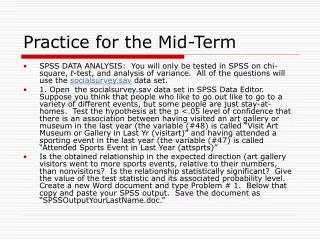
Practice for the Mid-Term • SPSS DATA ANALYSIS: You will only be tested in SPSS on chi-square, t-test, and analysis of variance. All of the questions will use the socialsurvey.sav data set. • 1. Open the socialsurvey.sav data set in SPSS Data Editor. Suppose you think that people who like to go out like to go to a variety of different events, but some people are just stay-at-homes. Test the hypothesis at the p <.05 level of confidence that there is an association between having visited an art gallery or museum in the last year (the variable (#48) is called “Visit Art Museum or Gallery in Last Yr (visitart)” and having attended a sporting event in the last year (the variable (#47) is called “Attended Sports Event in Last Year (attsprts)” • Is the obtained relationship in the expected direction (art gallery visitors went to more sports events, relative to their numbers, than nonvisitors? Is the relationship statistically significant? Give the value of the test statistic and its associated probability level. Create a new Word document and type Problem # 1. Below that copy and paste your SPSS output. Save the document as “SPSSOutputYourLastName.doc.”
Chi-Square: Appropriate Test for the Impact of a Nominal Level IV on another Nominal Level IV • To answer this question you will run a Chi-Square Analysis. You will be able to figure this out by first considering the level of measurement for the two variables. In the “Variable View” window look at the two variables, and note that each is measured not in terms of ranking or numeric values but in terms of discrete categories (whether they did or did not attend a sports event, and whether they did or did not visit a museum or gallery). For two nominal scale variables like this, the correct statistic to analyze their relationship would be Chi-square.
Running a Chi-Square Analysis in SPSS • Now that you have decided to run a Chi-square test, go to Analyze/Descriptives/Crosstabs • Move the Visited Art Galleries variable into the Columns box (you do this because the column variable is the one you are treating as independent, and in your hypothesis you have asked if there is a significant association between going to art galleries and going to sporting events). In the case of two variables like this there probably is no causal relationship, so which variable is the column variable is more or less arbitrary, but if your hypothesis were about the effect of say, gender, then gender is the obvious independent variable and would have to go in the column box) • Move the Attended Sport Events variable into the Rows box • Under Cells, click Observed, Expected, Row, Column and Total and click Continue (you do this so that you will have all the information you need to see if the direction of the relationship you predicted is in fact correct. In this case you want to know, is there an association between visiting art museums and going to sports events that is greater than what you might expect by chance)
How to Make Your Decisions • Under Statistics, click Chi-square, then Continue, and OK. (Chi-square is your test statistic) • To confirm your hypothesis, you need for the obtained value of Chi-square to be significant at the .05 level. SPSS will print out the exact probability level for you. You need for p to be less than .05 • However, if after getting a significant Chi-square you look over the table of observed versus expected counts and note that the trend is going in the wrong direction (that is, museum goers are less likely than expected to go to sports events) then although you can say that there may be an association, you have not established that more art visits are associated with more sporting event attendance.
Comparing Obtained (Count) to Expected (Expected Count) to Determine Direction of Relationship between the Two Variables On the right is what your output should look like for checking out the direction of the relationship. Note that within the group of art visitors that went to a sports event, the counter is higher than the expected count (orange), while within the group of non-visitors to art museums, the count of those who went to sports events is lower than the expected count (green). (The expected count for a cell is obtained in your SPSS output by multiplying the column total by the row marginal (see arrows). So your obtained results are in the direction you were expecting. Now it remains to be seen if this is a statistically significant relationship
Is the Obtained Value of Chi-square Significant? • Is the observed positive relationship between visiting a museum or gallery and attending a sports event statistically significant beyond the .05 level? According to the output, you have a chi-square of 79.414 (df = 1) which is significantly less likely than the .05 probability level. If it were not significant, the value in the fourth column below would read .051 or larger. • So it’s fair to say that you have confirmed the hypothesis there is a significant association between attending visiting art museums and visiting sporting events, and that the trend is for the relationship to be positive
Difference of Means Test for Two Levels of the IV: T Test • For the exam, we will only consider the t test for independent samples in doing an SPSS application. A t test is used when you have only two groups on the IV (two categories of a nominal-level independent variable, such as gender), and interval or ratio level for the DV • There are three varieties of t test in your SPSS list of options (independent, dependent or pairedsuch as pre-post comparisons, and single sample (such as comparing a sample mean to an assumed population mean or other known parameter) • Here’s a sample test question: Test the hypothesis that people with a college degree ((#59) “College Degree” (degree2) watch fewer hours of TV (the variable (#35) “Hours per Day Watching TV (tvhours)”) than people without a college degree. Test the hypothesis at the .01 level of confidence. Report the test statistic, df, probability level and the means for the two levels of the independent variable. Use the Levene test to determine which statistic you should report
Determine the Fit between Levels of Measurement of IV and DV and the Statistical Test • Look at the variables in Variable View. You see that the IV, college degree, has two categories and that it is a nominal level variable (ignore the “ordinal” tag that is attached to all of the variables in the data file; it is not true of all of them) because there are only two discrete categories, have the degree and don’t have the degree • Similarly, look at the DV, hours spent watching TV. This is at least an interval level measure. • Therefore, this question is suitable for the t test, which is for testing the impact of a two-level nominal level IV on variation in an interval or better DV (alternatively, testing whether the means on two “groups” (levels of the IV) differ significantly on the DV (are drawn from different populations)
Running a t Test for Independent Samples in SPSS • In Data Editor, go to Analyze/ Compare Means/ Independent Samples T-Test • Move the College Degree (degree2) variable into the Group Variable box and click on the Define button to assign values to levels of the variable. Use the values from the Variable View which assign 0 to Group 1 (no degree) and 1 to Group 2 (college degree) • Move the Hours Watching per Day Watching TV variable into the Test Variable(s) box • Under Options, set the confidence interval to 99% and click Continue, and then OK • Use your output to answer the question
Finding Answers to the Question in Your SPSS T Test Output First, check to see if the variances between the two groups in the IV are significantly different based on Levene’s statistic: they are (note the probability level which shows the statistic fell into the critical region). This determines which value of t you will report. The tests shows that you can’t assume equal variances (they are significantly different) so you have to use the value of t which is calculated assuming unequal variances: 12.275 Levene’s test shows signfiicant difference of variances between two levels of the IV
Answering Your Question • Here’s a way to write the answer: A test of the hypothesis that people with a college degree would differ from people without a college degree on number of hours spent per day watching TV indicated that there was a significant difference in number of hours spent watching TV (t (unequal variances) = 12.275, df = 1149.777, p < .0005) . (Note that since your test is one-tailed (you predicted a direction, you have to “cut the probability in half” since SPSS only reports the two-tailed test). Persons with a college degree spent an average of 1.99 hours per week watching TV while persons without a college degree spent an average of 3.17 hours per day watching TV. Here are the group means
Univariate Analysis of Variance: an Appropriate Test of the Impact of a 3- or More Level IV on an Interval or Ratio Level DV: Sample Problem • A Sample Problem for the Midterm: Test the hypothesis that religious preference of respondent (the variable (#27) “Religious Preference (relig)”) has a significant impact on hours per day watching TV (the variable (#35) “Hours per Day Watching TV (tvhours)”) Make a decision in advance to reject the null hypothesis (and confirm the research hypothesis) if the obtained value of the test statistic falls into the .01 confidence region
Sample Problem, cont’d • Write up your results as if you were writing for a journal. Include • The value of the test statistic • The degrees of freedom • The level of significance associated with the test statistic • Report the effect size (amount of variance accounted for, the partial eta squared) • The statistical power associated with your test • Report the results of the test for equality of variances • Report the means for each condition (level of the variable “religious preference”). • Run post hoc tests using Sheffe to see if there are significant pair-wise differences in mean TV hours watched among the levels of the independent variable (religious preference) and report which ones are significant. • If there is anything in your printout that suggests that the Sheffe tests might not be appropriate, run the more appropriate type of post-hoc test. Make an assessment as to the importance of the observed relationship between religious preference and hours watching TV based on the effect size
What Kind of Variables Do I Have? • First consult the Variable View in SPSS Data Editor to find out what kinds of variables these are (look under the value labels). You will see that religious preference is a nominal level variable with five categories, and tv hours is a ratio level variable. The appropriate analysis for studying the effect of a nominal level variable with more than two levels (categories) on an interval or ratio level variable is an analysis of variance (ANOVA). So you make the decision that you will run an ANOVA and treat religious preference as the IV and hours watching TV as the DV
Running ANOVA in SPSS • Go to Analyze/ General Linear Model / Univariate • Move the Religious Preference variable into the Fixed Factor(s) Window (this is where “fixed” IVs go) • Move the Hours Per Day Watching TV Variable into the Dependent Variable box (you are saying TV hours watched is “dependent” on religious preference) • Don’t make any changes under Model, Contrasts, or Plots • Under Options, move Overall, Relig to the Display Means window • Also under Options/Display, select descriptive statistics, estimates of effect size, observed power, and homogeneity tests. You know to ask for these because the question asked you to provide them. This will give you the mean tv hours according to religion, the effect size (how much variance in tv hours you can explain with religion), how much power you had to detect a difference if there is one, and whether or not your levels of the IV have different variances and thus you need to do the alternative tests (Tamhane, not Sheffe, for example) • Finally under Options set the significance level to .01 and click Continue
More ANOVA in SPSS • Click the Post Hoc Button and move relig into the Post Hoc Tests for window • Under equal variances assumed select Scheffe (you will use this test if the group variances do not differ significantly according to the Lehane test; Lehane test will show up on your output) • Under equal variances not assumed select Tamhane T2 test (you will use this test if the group variances are significantly different according to the Lehane test) • Click Continue and then OK • Consult your output to answer the question
Getting the Answers from Your SPSS Output: F, Significance, eta square, Power Here is the overall F statistic and its associated level of signifcance. It is not significant according to the .01 level you set up because the obtained value is larger than .01, so you can’t reject the null hypothesis DF Here are the partial eta squared (percent of variance in DV explained by the IV) and the power estimate
More Answers from the SPSS output: Means on the DV by Level of the IV; Equality of Variances Test Here are the group means which show how average hours watching TV varied as a function of religious preference. This table also gives you a numerical breakdown of the religious preference categories Here is the Levene test of equality of variances between levels of the IV, which in this case is significant beyond the .001 level. This means the variances can’t be assumed to be equal, so instead of the Sheffe post hoc tests you use a test like the Tamlane for unequal group variances
Post-hoc Comparisons when Equal Variances Can’t be Assumed Significance levels • If the overall effect is not significant the post-hoc pairwise comparisons probably won’t be (for example comparing Catholics to Protestants) but let’s look at the output anyhow. Look at the table in your output called Post Hoc Tests, Religious Preference, Multiple Comparison (the bottom half). We have already established that we have to use the post hoc tests which assume unequal group variances, so we will look only at the Tamhane tests in the bottom half of the table. Look at the column called Significance and you will see that none of the tests yields a value of significance less than .05
Answer to the Question: What your “Results” Section Would Say • Answer: To test the hypothesis that religious preference has a significant impact on hours spent watching TV, a one-way analysis of variance was conducted. The obtained value of F (4, 1478) of 2.664 was not significant at the .01 level. The effect size (partial eta squared) was .007. Power to detect the effect was .522. The Levene test for the equality of variances among the levels of the independent variable (religious preference) found that the variances were significantly different (F = 6.850, p < .001), suggesting that an alternative post hoc test for pair-wise differences of means should be used. The mean TV hours watched by religious preference were: Jewish, 2.45; “other,” 2.62; Catholic, 2.75; Protestant, 2.90; and “none,” 3.42. Tamhane tests of post-hoc differences indicated that there were no significant differences in TV hours watched between any levels of the independent variable. However, power to detect a between-groups effect was low (.522) despite the large sample size, so the issue might be revisited in a new study with more power to detect a small effect.