Chapter 3 FLUID-FLOW CONCEPTS AND BASIC EQUATIONS
Chapter 3 FLUID-FLOW CONCEPTS AND BASIC EQUATIONS. The statics of fluids: almost an exact science Nature of flow of a real fluid is very complex

Chapter 3 FLUID-FLOW CONCEPTS AND BASIC EQUATIONS
E N D
Presentation Transcript
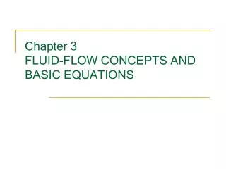
The statics of fluids: almost an exact science • Nature of flow of a real fluid is very complex • By an analysis based on mechanics, thermodynamics, and orderly experimentation, large hydraulic structures and efficient fluid machines have been produced. • This chapter: the concepts needed for analysis of fluid motion • the basic equations that enable us to predict fluid behavior (motion, continuity, and momentum and the first and second laws of thermodynamics) • the control-volume approach is utilized in the derivation of the continuity, energy, and momentum equations • in general, one-dimensional-flow theory is developed in this chapter
3.1 Flow Characteristics; Definitions • Flow: turbulent, laminar; real, ideal; reversible, irreversible; steady, unsteady; uniform, nonuniform; rotational, irrotational • Turbulent flow: most prevalent in engineering practice • the fluid particles (small molar masses) move in very irregular paths causing an exchange of momentum from one portion of the fluid to another • the fluid particles can range in size from very small (say a few thousand molecules) to very large (thousands of cubic meters in a large swirl in a river or in an atmospheric gust) • the turbulence sets up greater shear stresses throughout the fluid and causes more irreversibilities or losses • the losses vary about as the 1.7 to 2 power of the velocity; in laminar flow, they vary as the first power of the velocity.
Laminar flow: fluid particles move along smooth paths in laminas, or layers, with one layer gliding smoothly over an adjacent layer • governed by Newton's law of viscosity [Eq. (1.1.1) or extensions of it to three-dimensional flow], which relates shear stress to rate of angular deformation • the action of viscosity damps out turbulent tendencies • is not stable in situations involving combinations of low viscosity, high velocity, or large flow passages and breaks down into turbulent flow • An equation similar in form to Newton's law of viscosity may be written for turbulent flow: η: not a fluid property alone; depends upon the fluid motion and the density - the eddy viscosity. • In many practical flow situations, both viscosity and turbulence contribute to the shear stress:
An ideal fluid: frictionless and incompressible and should not be confused with a perfect gas • The assumption of an ideal fluid is helpful in analyzing flow situations involving large expanses of fluids, as in the motion of an airplane or a submarine • A frictionless fluid is nonviscous, and its flow processes are reversible. • The layer of fluid in the immediate neighborhood of an actual flow boundary that has had its velocity relative to the boundary affected by viscous shear is called the boundary layer • may be laminar or turbulent, depending generally upon its length, the viscosity, the velocity of the flow near them, and the boundary roughness • Adiabatic flow : no heat is transferred to or from the fluid • Reversible adiabatic (frictionless adiabatic flow): isentropic flow
Steady flow occurs when conditions at any point in the fluid do not change with the time • : ∂v/∂t = 0, space is held constant • no change in density ρ, pressure p, or temperature T with time at any point • Turbulent flow (due to the erratic motion of the fluid particles): small fluctuations occurring at any point; the definition for steady flow must be generalized somewhat to provide for these fluctuations: • Fig.3.1 (a plot of velocity against time, at some point in turbulent flow) • When the temporal mean velocity does not change with the time, the flow is said to be steady. • The same generalization applies to density, pressure, temperature • The flow is unsteady when conditions at any point change with the time, ∂v/∂t ≠ 0 • Steady: water being pumped through a fixed system at a constant rate • Unsteady: water being pumped through a fixed system at an increasing rate
Uniform flow: at every point the velocity vector is identically the same (in magnitude and direction) for any given instant • ∂v/∂s= 0, time is held constant and δs is a displacement in any direction : • no change in the velocity vector in any direction throughout the fluid at any one instant • says nothing about the change in velocity at a point with time. • In flow of a real fluid in an open or closed conduit: • even though the velocity vector at the boundary is always zero • when all parallel cross sections through the conduct are identical (i.e., when the conduit is prismatic) and the average velocity at each cross section is the same at any given instant, the flow is said to be uniform • Flow such that the velocity vector varies from place to place at any instant ∂v/∂s ≠ 0: nonuniform flow • A liquid being pumped through a long straight pipe has uniform flow • A liquid flowing through a reducing section or through a curved pipe has nonuniform flow.
Examples of steady and unsteady flow and of uniform and nonuniform flow • liquid flow through a long pipe at a constant rate is steady uniform flow • liquid flow through a long pipe at a decreasing rate is unsteady uniform flow • flow through an expanding tube at a constant rate is steady nonuniform flow • flow through an expanding tube at an increasing rate is unsteady nonuniform flow
Rotation of a fluid particle about a given axis, say the z axis: the average angular velocity of two infinitesimal line elements in the particle that are at right angles to each other and to the given axis • If the fluid particles within a region have rotation about any axis, the flow is called rotational flow, or vortex flow • If the fluid within a region has no rotation, the flow is called irrotational flow • If a fluid is at rest and is frictionless, any later motion of this fluid will be irrotational.
One-dimensional flow neglects variations of changes in velocity, pressure, etc., transverse to the main flow direction • Conditions at a cross section are expressed in terms of average values of velocity, density, and other properties • Flow through a pipe • Two-dimensional flow: all particles are assumed to flow in parallel planes along identical paths in each of these planes no changes in flow normal to these planes • Three-dimensional flow is the most general flow in which the velocity components u, v, w in mutually perpendicular directions are functions of space coordinates and time x, y, z, and t • Methods of analysis are generally complex mathematically, and only simple geometrical flow boundaries can be handled
Streamline: continuous line drawn through the fluid so that it has the direction of the velocity vector at every point • There can be no flow across a streamline • Since a particle moves in the direction of the streamline at any instant, its displacement δs, having components δx, δy, δz, has the direction of the velocity vector q with components u, v, w in the x, y, z directions, respectively : the differential equations of a streamline; any continuous line that satisfies them is a streamline
Steady flow (no change in direction of the velocity vector at any point): the streamline has a fixed inclination at every point - fixed in space • A particle always moves tangent to the streamline in steady flow the path of a particle is a streamline • In unsteady flow (the direction of the velocity vector at any point may change with time): a streamline may shift in space from instant to instant • A particle then follows one streamline one instant, another one the next instant, and so on, so that the path of the particle may have no resemblance to any given instantaneous streamline. • A dye or smoke is frequently injected into a fluid in order to trace its subsequent motion. The resulting dye or smoke trails are called streak lines. In steady flow a streak line is a streamline and the path of a particle.
Streamlines in two-dimensional flow can be obtained by inserting fine, bright particles (aluminum dust) into the fluid, brilliantly lighting one plane, and taking a photograph of the streaks made in a short time interval. Tracing on the picture continuous lines that have the direction of the streaks at every point portrays the streamlines for either steady or unsteady flow. • Fig. 3.2: illustration of an incompressible two-dimensional flow; the streamlines are drawn so that, per unit time, the volume flowing between adjacent streamlines is the same if unit depth is considered normal to the plane of the figure • when the streamlines are closer together, the velocity must be greater, and vice versa. If u is the average velocity between two adjacent stream-lines at some position where they are h apart, the flow rate Δq is • A stream tube : made by all the streamlines passing through a small, closed curve. In steady flow it is fixed in space and can have no flow through its walls because the velocity vector has no component normal to the tube surface
Figure 3.2 Streamlines for steady flow around a cylinder between parallel walls
Example 3.1 In two-dimensional, incompressible steady flow around an airfoil the streamlines are drawn so that they are 10 mm apart at a great distance from the airfoil, where the velocity is 40 m/s. What is the velocity near the airfoil, where the streamlines are 75 mm apart? and
3.2 The Concepts of System and Control Volume • The free-body diagram (Chap. 2): a convenient way to show forces exerted on some arbitrary fixed mass – a special case of a system. • A system refers to a definite mass of material and distinguishes it from all other matter, called its surroundings. • The boundaries of a system form a closed surface; it may vary with time, so that it contains the same mass during changes in its condition (for example, a kilogram of gas may be confined in a cylinder and be compressed by motion of a piston; the system boundary coinciding with the end of the piston then moves with the piston) • The system may contain an infinitesimal mass or a large finite mass of fluids and solids at the will of the investigator.
The law of conservation of mass: the mass within a system remains constant with time (disregarding relativity effects): m is the total mass. • Newton's second law of motion is usually expressed for a system as m is the constant mass of the system; ∑F refers to the resultant of all external forces acting on the system, including body forces such as gravity; v is the velocity of the center of mass of the system.
A control volume refers to a region in space and is useful in the analysis of situations where flow occurs into and out of the space • The boundary of a control volume is its control surface • The size and shape of the control volume are entirely arbitrary, but frequently they are made to coincide with solid boundaries in parts; in other parts they are drawn normal to the flow directions as a matter of simplification • By superposition of a uniform velocity on a system and its surroundings a convenient situation for application of the control volume may sometimes be found, e.g., determination of sound-wave velocity in a medium • The control-volume concept is used in the derivation of continuity, momentum, and energy equations. as well as in the solution of many types of problems • The control volume is also referred to as an open system.
Regardless of the nature of the flow, all flow situation are subject to the following relations, which may be expressed in analytic form: • Newton's laws of motion, which must hold for every particle at every instant • The continuity relation, i.e., the law of conservation of mass • The first and second laws of thermodynamics • Boundary conditions; analytical statements that a real fluid has zero velocity relative to a boundary at a boundary or that frictionless fluids cannot penetrate a boundary
Figure 3.3 System with identical control volume at time t in a velocity field
Fig.3.3: some general new situation, in which the velocity of a fluid is given relative to an xyz coordinate system (to formulate the relation between equations applied to a system and those applied to a control volume) • At time t consider a certain mass of fluid that is contained within a system, having the dotted-line boundaries indicated. • Also consider a control volume, fixed relative to the xyz axes, that exactly coincides with the system at time t. • At time t + δt the system has moved somewhat, since each mass particle moves at the velocity associated with its location. • N - the total amount of some property (mass, energy, momentum) within the system at time t;η - the amount of this property, per unit mass, throughout the fluid.The time rate of increase of N for the system is now formulated in terms of the control volume.
At t + δt, Fig. 3.3b, the system comprises volumes II and III, while at time t it occupies volume II, Fig. 3.3a. The increase in property N in the system in time δt is given by (*) • The term on the left is the average time rate of increase of N within the system during time δt. In the limit as δt approaches zero, it becomes dN/dt. • If the limit is taken as δt approaches zero for the first term on the right-hand side of the equation, the first two integrals are the amount of N in the control volume at t+δt and the third integral is the amount of N in the control volume at time t. The limit is
The next term, which is the time rate of flow of N out of the control volume, in the limit, may be written : dA, Fig 3.3c, is the vector representing an area element of the outflow area • Similarly, the last term of Eq. (*), which is the rate of flow of N into the control volume, is, in the limit, The minus sign is needed as v · dA (or cos α) is negative for inflow, Fig. 3.3d • Collecting the reorganized terms of Eq. (*) gives : time rate of increase of N within a system is just equal to the time rate of increase of the property N within the control volume (fixed relative to xyz) plus the net rate of efflux of N across the control-volume boundary
3.3 Application of The Control Volume to Continuity, Energy, and Momentum Continuity • The continuity equations are developed from the general principle of conservation of mass, Eq. (3.2.1), which states that the mass within a system remains constant with time, i.e. • In Eq. (3.2.6) let N be the mass of the system m. Then η is the mass per unit mass, : the continuity equation for a control volume : the time rate of increase of mass within a control volume is just equal to the net rate of mass inflow to the control volume.
Energy Equation • The first law of thermodynamics for a system: that the heat QH added to a system minus the work W done by the system depends only upon the initial and final states of the system - the internal energy E or by the above Eq.: • The work done by the system on its surroundings: • the work Wpr done by pressure forces on the moving boundaries • the work Ws done by shear forces such as the torque exerted on a rotating shaft. • The work done by pressure forces in time δt is
By use of the definitions of the work terms • In the absence of nuclear, electrical, magnetic, and surface-tension effects, the internal energy e of a pure substance is the sum of potential, kinetic, and "intrinsic" energies. The intrinsic energy u per unit mass is due to molecular spacing and forces (dependent upon p, ρ, or T):
Linear-Momentum Equation • Newton's second law for a system, Eq. (3.2.2), is used as the basis for finding the linear-momentum equation for a control volume by use of Eq. (3.2.6) • Let N be the linear momentum mv of the system, and let η be the linear momentum per unit mass ρv/ρ. Then by use of Eqs. (3.2.2) and (3.2.6) : the resultant force acting on a control volume is equal to the time rate of increase of linear momentum within the control volume plus the net efflux of linear momentum from the control volume. • Equations (3.3.1). (3.3.6), and (3.3.8) provide the relations for analysis of many of the problems of fluid mechanics - a bridge from the solid-dynamics relations of the system to the convenient control-volume relations of fluid flow
3.4 Continuity Equation • The use of Eq. (3.3.1) is developed in this section. First, consider steady flow through a portion of the stream tube of Fig. 3.4 The control volume comprises the walls of the stream tube between sections 1 and 2, plus the end areas of sections 1 and 2. Because the flow is steady, the first term of Eq. (3.3.1) is zero; hence : net mass outflow from the control volume must be zero • Since there is no flow through the wall of the stream tube : continuity equation applied to two sections along a stream tube in steady flow
Figure 3.4 Steady flow through a stream tube Figure 3.5 Collection of stream tubes between fixed boundaries
in which V1, V2 represent average velocities over the cross sections and m is the rate of mass flow. The average velocity over a cross section is given by • For a collection of stream tubes (Fig. 3.5), ρ1 is the average density at section 1 and ρ2 the average density at section 2, (3.4.3) • If the discharge Q (also called volumetric flow rate, or flow) is defined as (3.4.4) the continuity equation may take the form (3.4.5) • For incompressible, steady flow (3.4.6) • For constant-density flow, steady or unsteady, Eq. (3.3.1) becomes (3.4.7)
Example 3.2 At section 1 of a pipe system carrying water (Fig. 3.6) the velocity is 3.0 m/s and the diameter is 2.0 m. At section 2 the diameter is 3.0 m. Find the discharge and the velocity at section 2. From Eq. (3.4.6) and
Figure 3.7 Control volume for derivation of three-dimensional continuity equation in cartesian co-ordinates
For three-dimensional cartesian coordinates, Eq. (3.3.1) is applied to the control-volume element δx δy δz (Fig. 3.7) with center at (x, y, z), where the velocity components In the x, y, z directions are u, v, w, respectively, and ρ is the density. • Consider first the flux through the pair of faces normal to the x direction. On the right-hand lace the flux outward is since both ρ and u are assumed to vary continuously throughout the fluid. ρu δy δz is the mass flux through the center face normal to the x axis. The second term is the rate of increase of mass flux, with respect to x multiplied by the distance δx/2 to the right-hand face. On the left-hand lace The net flux out through these two faces is
which takes the place of the right-hand pan of Eq. (3.3.1). The left-hand part of Eq. (3.3.1) becomes, for an element • The other two directions yield similar expressions; the net mass outflow is • When these two expressions are used in Eq. (3.3.1), after dividing through by the volume element and taking the limit as δx δy δz approaches zero, the continuity equation at a point becomes (3.4.8) • For incompressible flowit simplifies to
then • In vector notation: with the velocity vector (3.4.11) • Equation (3.4.8) becomes (3.4.12) • Eq. (3.4.9) becomes (3.14.13) : the divergence of the velocity vector q - it is the net volume efflux per unit volume at a point and must be zero for incompressible flow • Two-dimensional flow: generally assumed to be in planes parallel to the xy plane, w=0, and ∂/∂z=0, which reduces the three-dimensional equations given for continuity
Example 3.3 The velocity distribution for a two-dimensional incompressible flow is given by Show that it satisfies continuity. In two dimensions the continuity equation is, from Eq. (3.4.9) Then and their sum does equal zero, satisfying continuity.
3.5 Euler's Equation of Motion Along a Streamline • In addition to the continuity equation: other general controlling equations - Euler's equation. • In this section Euler's equation is derived in differential form • The first law of thermodynamics is then developed for steady flow, and some of the interrelations of the equations are explored, including an introduction to the second law of thermodynamics. Here it is restricted to flow along a streamline. • Two derivations of Euler's equation of motion are presented • The first one is developed by use of the control volume for a small cylindrical element of fluid with axis aling a streamline. This approach to a differential equation usually requires both the linear-momentum and the continuity equations to be utilized. • The second approach uses Eq. (2.2.5), which is Newton's second law of motion in the form force equals mass times acceleration.
Figure 3.8 Application of continuity and momentum to flow through a control volume in the S direction
Fig. 3.8: a prismatic control volume of very small size, with cross-sectional area δA and length δs • Fluid velocity is along the streamline s. By assuming that the viscosity is zero (the flow is frictionless), the only forces acting on the control volume in the x direction are the end forces and the gravity force. The momentum equation [Eq․(3.3.8)] is applied to the control volume for the s component. (3.5.1) • The forces acting are as follows, since as s increases, the vertical coordinate increases in such a manner that cosθ=∂z/∂s. (3.5.2) • The net efflux of s momentum must consider flow through the cylindrical surface , as well as flow through the end faces (Fig. 3.8c). (3.5.3)
(3.5.4) (3.5.5) • To determine the value of m·t , the continuity equatlon (3.3.1) is applied to the control volume (Flg. 3.8d). • Substituting Eqs. (3.5.2) and Eq. (3.5.5) into equation (3.5.1) (3.5.6) • Two assumptions : (1) that the flow is along a streamline and (2) that the flow is frictionless. If the flow is also steady, Eq․(3.5.6) (3.5.7) • Now s is the only independent variable, and total differentials may replace the partials, (3.5.8)
3.6 The Bernoulli Equation • Integration of equation (3.5.8) for constant density yields the Bernoulli equation (3.6.1) • The constant of integration (the Bernoulli constant) varies from one streamline to another but remains constant along a streamline in steady, frictionless, incompressible flow • Each term has the dimensions of the units metre-newtons per kilogram: • Therefore, Eq. (3.6.1) is energy per unit mass. When it is divided by g, (3.6.2) • Multiplying equation (3.6.1) by ρ gives (3.6.3)
Each of the terms of Bernoulli's equation may be interpreted as a form of energy. • Eq. (3.6.1): the first term is potential energy per unit mass. Fig. 3.9: the work needed to lift W newtons a distance z metres is WZ. The mass of W newtons is W/g kg the potential energy, in metre-newtons per kilogram, is • The next term, v2/2: kinetic energy of a particle of mass is δm v2/2; to place this on a unit mass basis, divide by δm v2/2 is metre-newtons per kilogram kinetic energy
The last term, p/ρ: the flow work or flow energy per unit mass • Flow work is net work done by the fluid element on its surroundings while it is flowing • Fig. 3.10: imagine a turbine consisting of a vaned unit that rotates as fluid passes through it, exerting a torque on its shaft. For a small rotation the pressure drop across a vane times the exposed area of vane is a force on the rotor. When multiplied by the distance from center of force to axis of the rotor, a torque is obtained. Elemental work done is p δA ds by ρδA ds units of mass of flowing fluid the work per unit mass is p/ρ • The three energy terms in Eq (3.6.1) are referred to as available energy • By applying Eq. (3.6.2) to two points on a streamline, (3.6.4)
Figure 3.9 Potential energy Figure 3.10 Work done by sustained pressure
Example 3.4 Water is flowing in an open channel (Fig. 3.11)at a depth of 2 m and a velocity of 3 m/s. It then flows down a chute into another channel where the depth is 1 m and the velocity is 10 m/s. Assuming frictionless flow, determine the difference in elevation of the channel floors. The velocities are assumed to be uniform over the cross sections, and the pressures hydrostatic. The points 1 and 2 may be selected on the free surface, as shown, or they could be selected at other depths. If the difference in elevation of floors is y, Bernoulli's equation is Thus and y = 3.64 m
Modification of Assumptions Underlying Bernoulli's Equation • Under special conditions each of the four assumptions underlying Bernoulli's equation may be waived. • When all streamlines originate from a reservoir, where the energy content is everywhere the same, the constant of integration does not change from one streamline to another and points 1 and 2 for application of Bernoulli's equation may be selected arbitrarily, i.e., not necessarily on the same streamline. • In the flow of a gas, as in a ventilation system, where the change in pressure is only a small fraction (a few percent) of the absolute pressure, the gas may be considered incompressible. Equation (3.6.4) may be applied, with an average unit gravity force .
For unsteady flow with gradually changing conditions, e.g., emptying a reservoir, Bernoulli's equation may be applied without appreciable error. • Bernoulli's equation is of use in analyzing real-fluid cases by first neglecting viscous shear to obtain theoretical results. The resulting equation may then be modified by a coefficient, determined by experiment, which corrects the theoretical equation so that it conforms to the actual physical case. In general, losses are handled by use of the energy equation developed in Secs. 3.8 and 3.9.