Class 9 March 23, 2006
570 likes | 808 Vues
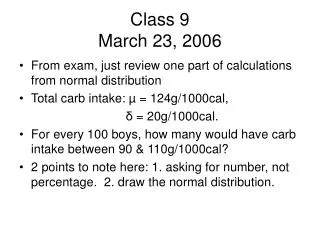
Class 9 March 23, 2006. From exam, just review one part of calculations from normal distribution Total carb intake: µ = 124g/1000cal, δ = 20g/1000cal. For every 100 boys, how many would have carb intake between 90 & 110g/1000cal?

Class 9 March 23, 2006
E N D
Presentation Transcript
Class 9March 23, 2006 • From exam, just review one part of calculations from normal distribution • Total carb intake: µ = 124g/1000cal, δ = 20g/1000cal. • For every 100 boys, how many would have carb intake between 90 & 110g/1000cal? • 2 points to note here: 1. asking for number, not percentage. 2. draw the normal distribution.
Review estimate of the mean Confidence intervals, that is, what is the probability that a population mean will fall within a certain range based on an estimate using a sample mean.
Usual Intervals • Usually use 90%, 95% or 99% • What are the corresponding Z values? • For now, start with 95% • Last time we found that Z = 1.96 • Just accept that for the moment; we will review how to get it shortly.
Example Estimate the mean birth weight of newborns with gestational age 40 weeks, based on a sample of 5 such newborns with a mean birth weight of 3500 grams and a standard deviation of 430 grams. Since there are only 5 in the sample, what do we have to assume? Have to assume that the population from which the sample is drawn is approximately normal and that these are 5 randomly chosen newborns.
Always draw the N.D. The shaded area can help us to see what we mean by It is the border of the shaded area to the right of the mean . We are saying that the mean lies between that border and the corresponding left-side border
Write the equation Mu lies between the two values within the parentheses
Practical Statement of Result • With 95% confidence, we can say that u will be ≤ 1.96 *S.E. and • ≥ -1.96 * S.E. • We call 1.96 the reliability coefficient
The Math • X = 3500 g, n = 5, б = 430 • Review what the symbols mean • Find the quantity б / Γn = 430/ Γ5 = 430/ 2.24 = 192 • 1.96 * 192 = 376 • Mu is between 3500 – 376 and 3500 + 376 • 3124 ≤ µ≤ 3876 with 95% confidence
How did we get Z • Review for 95% what is the area not included divide into 2 tails look up Z • Try for 90% • Try for 99%
Applications • If we know a population mean & st. dev., we can calculate the probability that any sample will have a stated mean. • A certain large human pop’n has a cranial length that is approx’ly normally distributed with mean 185.6 mm and б of 12.7 mm.
µ = 185.6 mm б = 12.7 mm • What is the probability that a random sample of size 10 from this population will have a mean greater than 190? • We can calculate this probability but why would we?
Usefulness?? • Let’s say that it is accepted knowledge that the population has a certain mean. • I am working with a group of people. • I want to know if they fit into this population with regard to the particular parameter. If the probability of the mean of the sample is very low, perhaps it is not really from the same population
Education Example • Third-graders in the U.S. have an average reading score of 124. • Third-graders in a particular school have a mean reading score of 120. What’s the probability that they are from the same population?
Back to Cranial Length • µ = 185.6 mm б = 12.7 mm • random sample of size 10 from this population will have a mean greater than 190? • Have to find how far 190 is from 185.6 in units of standard error of the mean
0.138 185.6 190 0 1.09 Probability of Mean of 190 Did you draw a normal dist??? Z = 4.4 / 12.7 / 3.16 Z = 1.09 Area = 0.138 The probability is 13.8%
Hypothesis Testing A frequently used method in clinical research
Another Look at Confidence Intervals • 95% C.I.: The space in each tail is 0.025. • The sum is 0.050 • This value, the space not covered in the C.I., is called alpha. • α is called the Significance Level • Each tail contains α/2
Using a Confidence Interval • A school district administrator took sample(s) of fifth grade reading scores for all the schools in Nassau County and then estimated a 90% C.I. for the mean: 87.60 to 92.34 with a sigma of 10. • All the individual schools then compared their mean to this. • If they did not fall within the interval, they were considered significantly better or significantly worse and faculty hiring's were affected by the results.
Hypothesis Testing Just a new way to ask the questions. The methods used are virtually the same as C.I.’s
The More Usual Approach • The most frequent application of estimating the mean is to look for effects that put a group outside the interval . • We usually set up research so that we are looking for a difference
A New Drug to Lower Cholesterol • Everyone has been using my competitors product named reductum • I have developed a drug called drasticchangum • I want to find out if my product has results different from the accepted treatment
Set Up a Hypothesis • My hope is that there is a difference between my product and theirs. • I set up Hypothesis A that says there is a difference • In order to test it, I state another hypothesis saying that there is NO DIFFERENCE between the 2 treatments. • I want to reject this hypothesis
Another Wording • HA says that the sample comes from a population with a mean different from that of the original population • H0 says that the sample comes from a population with a mean the same as that of the original population. We call this µ0
The Hypothesis to Reject • This is called the Null Hypothesis, H0 • I now go about the process to reject it. • I have to choose a significance level • Let’s say α = 0.01, analogous to a C.I. of 99%
Set-Up • Each tail has probability of α/2. Call it Rejection Zone • For α = 0.01, each tail has 0.005 and this occurs for any Z that is over 2.54 Check the table of Normal Distribution
Results • The population treated by reductum has a mean change in cholesterol of 30 units with a sigma of 4.5. • I have a preliminary sample of 10 patients treated by drasticchangum. Their mean change is 34 units. I assume that they come from a population that has the same sigma as the first.
Hypotheses • HA: Called the Alternative Hypothesis. This is the result I want to support: “µ for the new population differs from 30. µ ≠ 30.” • H0: The Null Hypothesis, I want to reject this: µ for the new population is the same as the old, that is 30. “µ = 30”.
The Test Statistic • Z = (X - µ0) / б/Γn • Z = (34 – 30) / 4.5 / Γ10 • Z = 2.81 • This is larger than 2.54 so is in the rejection zone
Excellent Result • We can reject the null hypothesis • We can accept the alternative hypothesis • I can say that drasticchangum causes a different change in cholesterol level from reductum. • Is there anything else we might prefer to say? • How about “Drasticchangum causes a greater change than does reductum.”?
Different Hypotheses • HA: The mean for DC is greater than 30. • H0 : The mean for DC is equal to 30 • How can we reject H0?
One-Sided Tests • So far we have divided alpha into the two tails. • Let’s put the whole alpha into just one tail. • Can we still reject the null hypothesis at the level of α = 0.01 (99% confidence)? • Look up the tail with area = 0.01 • Now Z just has to exceed 2.30. • It’s even easier to reject
Easier to Reject • If we choose the correct side to consider then it is easier to reject the null hypothesis • And accept the alternative hypothesis • Remember to express the correct alternative hypothesis before starting the math.
The Two Things We Can Say • We reject the null hypothesis that the sample came from the original population • We accept the alternative hypothesis that the sample came from a population with a mean greater than that of the original population.
So…Nothing so new • Hypothesis Testing is a cinch – because you already knew most of it from Confidence Intervals of the Normal Distribution • Let’s just look at some details
Confidence • Not only are we saying that drasticchangum has a greater effect than does reductum • But we have a level of significance, i.e. a statement of probability that we are correct. • But that means our conclusion could also be incorrect in reality even while satisfying our statistical conditions.
Possible Errors • In our example, we stated that the new sample came from a different population than the original • We could be incorrect. • What are the chances that we have stated a difference when there isn’t one? • The probability that the sample came from the old population is 0.01
Rejection Zone • If the new sample had a population mean equal to the original mean, there is only a 0.01 possibility that the sample mean would fall far enough from µ0 to give a Z of 2.30. • This would be a rare event but a possible one.
Type I Error • If we say that there is a difference when there really isn’t one. That is called a Type I Error. • We were statistically allowed to reject the null hypothesis but only some spiritual being somewhere knew that we shouldn’t have done so. • We may never know that the result was incorrect or … • After 1000 patients have tried drasticchangum, we may find that it came from a population with a mean the same as that of reductum.
OR… • We may be able to state the probability even more precisely. • The value of “p”. • Use the value calculated for Z, 2.81 • The area under the tail of the Normal Distribution is 0.002 • The chance that the means are equal is equal to or less than 0.002 • A report would state p ≤ 0.002
Conclusion • The null hypothesis is rejected with a p value less than or equal to 0.002 • The alternative hypothesis is accepted stating that the effect of drasticchangum is greater than that of reductum.
An Example • Weight Watchers Inc claims that those who have followed their program for at least a yr maintain some weight loss even after they have left the formal program. • A competitive group claims that those who have left the program have a rebound effect and actually weigh more than they would have if they had never tried the ww program
Before Gathering Data • HA: there is a difference between the average for former weight watchers and the general population • H0: The mean weight for both groups is the same. µest = µ0 • Test the null hypothesis with a significance level of 0.05 • Is the test one-sided or two-sided?
Are the Wts different from the general population • Considering the population of women from ages 30 to 60, it is accepted that the average weight is 150 with a variance of 20 lbs. • A sample of 20 former weight watchers have an average weight of 147 pounds
Establish Zcrit & determine Zcalc • For α = 0.05, & a 2-sided test, what is Zcrit? • Check the table for area of 0.025. Z = 1.96 • Zcalc = (147-150)/Γ20/ Γ20 = 3/ Γ1 = 3 • Do we reject the null hypothesis? • Do we accept the alternative hypothesis? • Yes to both and what is p? • p ≤ 0.001
Review p • We got p by looking up the area corresponding to a Zcalc of 3.0. Check it. • What does it mean that p ≤ 0.001? • It means that the chance of a Type I error is ≤ 0.001. • It means that the chance that the sample came from the population with mean of 150 is ≤ 0.001
Could we have set up a different test? • Yes, we could have asked a one-sided type question. • How would WW Inc have asked the question? • One-sided: WW average is less than population • Is there an advantage for them in choosing this? • Yes, a one-sided test would have given a greater area in the rejection zone. • Easier for them to show that their former clients weigh less than the overall population • Would p be any different? • No. What is different? • Zcrit
Another Sample • A pharmaceutical company says that it is more effective to take a weight loss drug. • They say they have a sample of 100 former weight watchers with an average weight of 149.5. • Now do a two-sided test on this.
Zcalc = (149.5-150)/Γ20/ Γ100 = 0.5/ Γ0.5 = 0.7 • Can we reject the null hypothesis? • No • Can we accept the null hypothesis that the average weight of the former ww’s equals the general population? • NO, NO, NO, NO, NO, NO • We never accept the null hypothesis • All we can say is – not enough evidence to reject.
