New Compression Codes for Text Databases
Laboratorio de Bases de Datos Universidade da Coruña. New Compression Codes for Text Databases. Ph.D. Dissertation Antonio Fariña Martínez. Advisors. Nieves R. Brisaboa Gonzalo Navarro. A Coruña. April 28th, 2005. Outline. Outline. Introduction. Two Scenarios. Semi-static Compressors

New Compression Codes for Text Databases
E N D
Presentation Transcript
Laboratorio de Bases de Datos Universidade da Coruña New Compression Codes for Text Databases Ph.D. Dissertation Antonio Fariña Martínez Advisors Nieves R. Brisaboa Gonzalo Navarro A Coruña. April 28th, 2005
Outline Outline • Introduction • Two Scenarios • Semi-static Compressors • Word-based Huffman:Plain & Tagged Huffman • End-Tagged Dense Code • (s,c)-Dense Code • Empirical Results • Dynamic Compressors • Statistical Dynamic compressors • Word-based Huffman • Dynamic End-Tagged Dense Code • Dynamic (s,c)-Dense Code • Empirical Results • Conclusions and Contributions of the Thesis
Introduction • In the last years … • Increase of number of text collections and their size • The Web, text databases (jurisprudence, linguistics, corporate data) • Compression reduces: • Storage space • Disk access time • Transmission time • Applications • Efficient retrieval. Searches can be even faster than in plain text • Transmission of data (and also real time transmission) • …
Introduction • Importance of compression in Text Data Bases • Reduces their size: 30% compression ratio • It is possible to search the compressed text directly • Searches are up to 8 times faster. • Decompression is only needed for presenting results • Compression can be integrated into Text Retrieval Systems, improving their performance • …
Introduction • Statistical compressors • Computation of the frequencies of the source symbols • More frequent symbols shorter codewords • A varying length codeword is given to each symbol Obtain compression • Two big families of compressors • Dictionary-based (gzip, compress,… ) • Statistical compressors (Huffman-based, arithmetic, PPM,… )
Outline Outline • Introduction • Two Scenarios • Semi-static Compressors • Word-based Huffman: Plain & Tagged Huffman • End-Tagged Dense Code • (s,c)-Dense Code • Empirical Results • Dynamic Compressors • Statistical Dynamic compressors • Word-based Huffman • Dynamic End-Tagged Dense Code • Dynamic (s,c)-Dense Code • Empirical Results • Conclusions and Contributions of the Thesis
Scenarios • 2 scenarios • Semi-static compression (2-pass) • Text storage • Text Retrieval • Dynamic compression (1-pass) • Transmission of data • Transmission of streams
Outline Outline • Introduction • Two Scenarios • Semi-static Compressors • Word-based Huffman: Plain & Tagged Huffman • End-Tagged Dense Code • (s,c)-Dense Code • Empirical Results • Dynamic Compressors • Statistical Dynamic compressors • Word-oriented Huffman • Dynamic End-Tagged Dense Code • Dynamic (s,c)-Dense Code • Empirical Results • Conclusions and Contributions of the Thesis
Semi-static compression • Statistical compression • 2 passes • Gather frequencies of source symbols and encoding • Compression (substitution source symbol codeword)
Semi-static compression de 2 C 1 no 2 C 2 En 1 C 3 un 1 C 4 lugar 1 C 5 la 1 C 6 Mancha 1 C 7 cuyo 1 C 8 nombre 1 C 9 quiero 1 C 10 acordarme 1 C 11 1st pass: Text processing > Vocabulary sorting > Code generation codeword vocabulary 1 En un lugar de la Mancha de 1 cuyo nombre 1 no quiero 1 2 acordarme no 1 … 1 1 Source text 1 1 2 1 1
Semi-static compression C C 1 3 C C 2 4 C C 3 5 header de*no*En*… C C C 4 1 1 C C 6 5 … C C 7 6 C C 7 8 C C 9 8 C C C 2 9 2 C C 10 10 C C 11 11 2nd pass: Substitution word codeword vocabulary codeword de 2 no 2 En 1 un 1 En un lugar de la mancha de lugar 1 cuyo nombre la 1 Compr. data no quiero Mancha 1 acordarme no cuyo 1 … nombre 1 Output file Source text quiero 1 acordarme 1
Semi-static compression • Statistical compression • 2 passes • Gather frequencies of words and encoding • Compression (substitution word codeword) • Association between source symbol codeword does not change across the text • Direct search is possible • Most representative method: Huffman.
Classic Huffman Building a Huffman tree • Optimal prefix code (i.e., shortest total length) • Character based (originally) • Characters are the symbols to be encoded • Bit oriented: Codewords are sequences of bits • A Huffman tree is built to generate codewords • Sorting symbols by frequency
Building a Huffman tree • Bottom-up construction 0.30 D E 0.15 0.15
Building a Huffman tree • Bottom-up construction 0.45 0.30 B C 0.25 0.20 D D E E 0.15 0.15
Building a Huffman tree • Bottom-up construction 0.55 0.45 0.30 A B B C C 0.25 0.25 0.20 D D D E E E 0.15 0.15
Building a Huffman tree • Bottom-up construction 1.00 0.55 0.45 0.30 A B C 0.25 0.25 0.20 D E 0.15 0.15
Building a Huffman tree 0 1 A B C D E • Labelling branches 1.00 0.55 0.45 0.30 A B B C C 0.25 0.25 0.20 D D D E E E 0.15 0.15
Building a Huffman tree 0 1 0 0 1 1 0 A B C 1 D E • Labelling branches 1.00 0.55 0.45 0.30 0.25 0.25 0.20 0.15 0.15
Building a Huffman tree • Code Assignment 1.00 0 1 0.55 0.45 0 0 1 1 0.30 0 A B C 1 0.25 0.25 0.20 D E 0.15 0.15 10 11 000 01 001
Building a Huffman tree 0 1 0 0 1 1 0 A B C 1 D E Ex: encoding ADB • Code Assignment 1.00 0.55 0.45 0.30 0.25 0.25 0.20 0.15 0.15 01 000 10
Classic Huffman • Optimal prefix code (i.e., shortest total length) • Character based (originally) • Characters are the symbols to be encoded • Bit oriented: Codewords are sequences of bits • A Huffman tree is built to generated codewords • Huffman tree has to be stored with the compressed text • Compression ratio about 60% (unpopular).
Outline Outline • Introduction • Two Scenarios • Semi-static Compressors • Word-based Huffman: Plain & Tagged Huffman • End-Tagged Dense Code • (s,c)-Dense Code • Empirical Results • Dynamic Compressors • Statistical Dynamic compressors • Word Oriented Huffman • Dynamic End-Tagged Dense Code • Dynamic (s,c)-Dense Code • Empirical Results • Conclusions and Contributions of the Thesis
Word-based Huffman Character freq distribution (Spanish) Word freq distribution • Moffat proposed the use of words instead of characters as the coding alphabet • Distribution of words more biased than the distribution of characters • Compression ratio about 25% (English texts) • This idea joins the requirements of compression algorithms and of Information Retrieval systems
Plain Huffman & Tagged Huffman • “1” for 1st bit of 1st byte • “0” for 1st bit remainingbytes First bit is: 1xxxxxxx 0xxxxxxx 0xxxxxxx • Moura, Navarro, Ziviani and Baeza: • 2 new techniques: Plain Huffman and Tagged Huffman • Common features • Huffman-based • Word-based • Byte- rather than bit-oriented (compression ratio ±30%) • Plain Huffman = Huffman over bytes (256-ary tree) • Tagged Huffman flags the beginning of each codeword
Plain Huffman & Tagged Huffman • Differences: • Plain Huffman. (tree of arity 2b=256) • Tagged Huffman. (tree of arity 2b-1 =128) • Loss of compression ratio (3.5 perc. points) • Tag marks beginning of codewords Direct search (searches improved) • Boyer-Moore Random access (random decompression)
Plain Huffman & Tagged Huffman: searches TAGGED HUFFMAN PLAIN HUFFMAN be 00 be 10 or 01 or 11 00 not 10 not 11 01 00 lucky 11 00 lucky 11 01 01 00 to 11 11 to 11 01 01 01 Searching for “lucky” to be lucky or not 1101010110 110101001100 110100 to be lucky or not 1111 001100 01 10 False matchings impossible False matching • Searches are improved Direct searching (compress pattern and search for it) Boyer-Moore type searching is possible (skipping bytes) to be lucky or not • Example (b=2):
Outline Outline • Introduction • Two Scenarios • Semi-static Compressors • Word-based Huffman: Plain & Tagged Huffman • End-Tagged Dense Code • (s,c)-Dense Code • Empirical Results • Dynamic Compressors • Statistical Dynamic compressors • Word-oriented Huffman • Dynamic End-Tagged Dense Code • Dynamic (s,c)-Dense Code • Empirical Results • Conclusions and Contributions of the Thesis
End-Tagged Dense Code • “1” --> for 1st bit of last byte • “0” --> for 1st bit remaining bytes 1xxxxxxx First bit is: 0xxxxxxx Two-byte codeword Three-byte codeword 0xxxxxxx 0xxxxxxx 1xxxxxxx 0xxxxxxx 1xxxxxxx Small change: Flag signal the end of a codeword Prefix code independently of the remaining 7 bits of each byte Huffman tree is not needed: Dense coding Flag bit Same Tagged Huffman searching capabilities
End-Tagged Dense Code 10000000 10000001 ….. 11111111 First 128 words are encoded using one byte (27codewords) 00000000:10000000 ….. 01111111:11111111 Words from 128+1 to 128+1282 are encoded using two bytes (1282 = 214codewords) 00000000:00000000:10000000 …… 01111111:01111111:11111111 Words from 128+ 1282+1 to 128 +1282 +1283 use three bytes (1283 = 221codewords) ..... • Encoding scheme • Codewords depend on the rank, not on the frequency
End-Tagged Dense Code • Sorting words by frequency • Code assignment Ci encode(i) i decode(Ci) ... 0xxxxxxx 0xxxxxxx 1xxxxxxx < 2b-1 < 2b-1 ≥ 2b-1 • On-the-fly encoding procedure • Sequential encoding procedure
End-Tagged Dense Code C 2 C 3 C 4 header de*no*En*… C C 0 0 vocabulary C 5 En un lugar de de 0 … la mancha de C 6 no 1 cuyo nombre C 7 En 2 no quiero C 8 un 3 acordarme no C C 1 1 lugar 4 … C 9 la 5 Plain text file C 10 • Decompression: two steps • Load the ranked vocabulary • i decode(Ci) Compr. data Compressed file …
End-Tagged Dense Code • It is a dense code. All the available codes can be used. • Compresses better than TH (2 percentage points). • It is overcome by PH (1 percentage point). • Flag same search capabilities than Tagged Huff. • direct search, • random access. • Efficient encoding and decoding • Sequential and on-the-fly procedures • Easy to program
Outline Outline • Introduction • Two Scenarios • Semi-static Compressors • Word-based Huffman: Plain & Tagged Huffman • End-Tagged Dense Code • (s,c)-Dense Code • Empirical Results • Dynamic Compressors • Statistical Dynamic compressors • Word-oriented Huffman • Dynamic End-Tagged Dense Code • Dynamic (s,c)-Dense Code • Empirical Results • Conclusions and Contributions of the Thesis
(s,c)-Dense Code • End Tagged Dense Code • 27 available values [128, 255] for last byte (stoppers) • 27 available values [0, 127] for other bytes (continuers) Why using fixed s,c values ? • Adapting s,c values to the vocabulary s minimizing compr. text size • number of words • distribution of frequency of the words • End-Tagged Dense Code is a (128,128)-Dense Code
(s,c)-Dense Code 0 ... s-1 s more frequent words s s ... s+c-1 0 1 ... s-1 Words from s+1 to s + sc (total sc words) Words from s + sc + 1 to s + sc + sc2 (total sc2 words) 0 ... s ... s ... • Stoppers: last byte. Values in [0,s-1] • Continuers: other bytes. Values in [s,s+c-1] • Encoding scheme
(s,c)-Dense Code • Example (b=3) Word Freq P.H. (6,2)-DC (5,3)-DC (4,4)- DC PH (6,2) (5,3) ETDC A 0,20 [000] 0,20 0,20 0,20 0,20 [000] [000] [000] B 0,20 [001] 0,20 0,20 0,20 0,20 [001] [001] [001] C 0,15 [010] 0,15 0,15 0,15 0,15 [010] [010] [010] D 0,15 [011] 0,15 0,15 0,15 0,15 [011] [011] [011] E 0,14 [100] 0,14 0,14 0,14 0,28 [100][000] [100] [100] F 0,09 [101] 0,09 0,09 0,18 0,18 [100][001] [101] [101][000] G 0,04 [110] 0,04 0,08 0,08 0,08 [100][010] [110][000] [101][001] H 0,02 [111][000] 0,04 0,04 0,04 0,04 [100][011] [110][001] [101][010] I 0,005 [111][001] 0,01 0,01 0,01 0,01 [101][000] [110][010] [101][011] J 0,005 [111][010] 0,01 0,01 0,01 0,01 [101][001] [110][011] [101][100] Average codeword lenght 1,03 1,07 1,16 1,30 • End-Tagged Dense Code is a (2b-1,2b-1)-DC
(s,c)-Dense Code ... xxxxxxxx xxxxxxxx zzzzzzzz s≤ vc< 2b-1 s≤ vc< 2b-1 0≤ vs< s • On-the-fly encoding is also possible • Sequential encoding Ci encode(s, i) i decode(s, Ci)
(s,c)-Dense Code • It is a dense code • Compresses better than TH (3 percentage points) • Compresses better than ETDC (0.75 percentage points) • It is overcome by PH (0.25 percentage point) • RATIO: PH < SCDC << ETDC <<< TH • Flag? (byte value < s) • Same search capatilities than End-Tagged Dense Code and Tagged Huffman • Simple encoding and decoding
Outline Outline • Introduction • Two Scenarios • Semi-static Compressors • Word-based Huffman: Plain & Tagged Huffman • End-Tagged Dense Code • (s,c)-Dense Code • Empirical Results • Dynamic Compressors • Statistical Dynamic compressors • Word-oriented Huffman • Dynamic End-Tagged Dense Code • Dynamic (s,c)-Dense Code • Empirical Results • Conclusions and Contributions of the Thesis
Empirical Results • We used some text collections from TREC-2 & TREC-4, to perform thorough experiments • Methods compared • Plain Huffman & Tagged Huffman • End-Tagged Dense Code • (s,c)-Dense Code • Comparison in: • Compression ratio • Encoding speed • Compression speed • Decompression speed • Search speed • Dual Intel Pentium-III 800 Mhz with 768Mb RAM. • Debian GNU/Linux (kernel 2.2.19) • gcc 3.3.3 20040429 and –O9 optimizations • Time represents CPU user-time
Compression Ratio (s,c)-DC ETDC TH PH 30.73 30.88 31.56 34.16 • In general PH (s,c)-DC ETDC < TH < < 0.2 pp 0.8 pp 2.5 pp
Compression time & encoding time 1st pass compression 2nd pass
Encoding time (s,c)-DC ETDC TH PH 260 143 104 270 • In general ETDC < (s,c)-DC < PH < TH 25% 45% 2%
Compression speed (s,c)-DC ETDC TH PH 5.92 5.88 5.90 5.83 • In general PH = ETDC > (s,c)-DC > TH
Decompression speed ETDC TH 23.86 23.55 24.15 22.51 (s,c)-DC PH • In general ETDC PH (s,c)-DC TH = > > 1.5% 4%
Search time (s,c)-DC ETDC TH PH 2.30 1.70 1.80 2.00 • 3-byte codes (s,c)-DC ETDC TH PH < < < 5% 5-10% 10% • Random patterns (n↑↑ ) TH overcomes (s,c)-DC ≈ 10%
Semi-static compression: Summary • Two new semi-static “dense” compressors: ETDC, SCDC • Simpler and faster encoding scheme than Huffman-based ones • Sequential encoding • on-the-fly encoding • Allowing direct search and random access • Speed: Good compression and decompression speed • Compression ratio close to Plain Huffman • Overcoming Tagged Huffman in: • Compression ratio, compression speed, decompression speed and searches.
Outline Outline • Introduction • Two Scenarios • Semi-static Compressors • Word-based Huffman: Plain & Tagged Huffman • End-Tagged Dense Code • (s,c)-Dense Code • Empirical Results • Dynamic Compressors • Statistical Dynamic compressors • Word-oriented Huffman • Dynamic End-Tagged Dense Code • Dynamic (s,c)-Dense Code • Empirical Results • Conclusions and Contributions of the Thesis