Stream Codes for Data Compression
Stream Codes for Data Compression. Yehong , Wang Wei, Wang Sheng, Jinyang , Gordon. Outline. Introduction Overview of Huffman Coding Arithmetic Coding Encoding and Decoding Probabilistic Model (break) Loss Analysis Lempel-Ziv Coding Summary. Why Data Compression?.

Stream Codes for Data Compression
E N D
Presentation Transcript
Stream Codesfor Data Compression Yehong, Wang Wei, Wang Sheng, Jinyang, Gordon
Outline • Introduction • Overview of Huffman Coding • Arithmetic Coding • Encoding and Decoding • Probabilistic Model (break) • Loss Analysis • Lempel-Ziv Coding • Summary
Why Data Compression? • Make optimal use of limited storage space • Save time and help to optimize resources • In sending data over communication line: less time to transmit and less storage to host
Data Compression • Encoding information using fewer bits than the original representation Data Compression Lossless methods (text, image) Lossy methods (audio, video, image) MPEG MP3 Arithmetic Lempel-Ziv Huffman JPEG
Outline • Introduction • Overview of Huffman Coding • Arithmetic Coding • Encoding and Decoding • Probabilistic Model (break) • Loss Analysis • Lempel-Ziv Coding • Summary
Huffman Coding • The key idea • Assign fewer bits to symbols that occur more frequently • Assign more bits to symbols appear less often • Algorithm: • Make a leaf node for each code symbol • Add the generation probability of each symbol to the leaf node • Take the two leaf nodes with the smallest probability and connect them into a new node • Add 1 or 0 to each of the two branches • The probability of the new node is the sum of the probabilities of the two connecting nodes • If there is only one node left, the code construction is completed. If not, go back to (2)
Huffman Coding • Example: 0.44 0.44 0.20 d b e a a a a a c d d d b b c c c c b d b b d e e e e e 0.08 0.08 0.08 0.08 0.08 0.12 0.24 0.24 0.25 0.24 0.31 0.31 0.31 0.31 0.31 0.25 0.12 0.12 0.12 0.12 0.25 0.24 0.25 0.25 0.24 a c (a) (d) (c) (b) (d) a: 000 b: 10 c: 001 d: 01 e: 11 1.00 1 0 0.56 1 0 0 1 0 1
Huffman Coding For an ensemble, the Huffman algorithm produces an optimal symbol code
Disadvantages of Huffman Coding For an ensemble, the Huffman algorithm produces an optimal symbol code • Unchanging ensemble: Huffman code is optimal • In practical, ensemble changes • Brute-force approach: recompute • Code remain fixed: suboptimal
Disadvantages of Huffman Coding For an ensemble, the Huffman algorithm produces an optimal symbol code • Unchanging ensemble: Huffman code is optimal • In practical, ensemble changes • Brute-force approach: recompute • Code remain fixed: suboptimal • Symbol code: encode one source symbol at a time • At least one bit per character • Extra bit problem
Disadvantages of Huffman Coding • The extra bit • Long strings of characters maybe highly predictable • For example: in the context “strings of ch”, one might predict the next symbols to be ‘aracters’ with a probability of 0.99 • Traditional Huffman code : at least one bit per character • For ‘aracters’, 8 bits, but no information is being conveyed
Data Compression Lossless methods (text, image) Lossy methods (audio, video, images) • Stream code: • encode huge strings of N source symbols • dispenses with the restriction that each symbol must be translated into an integer number of bits Symbol code: encode one source symbol at a time MPEG MP3 Arithmetic Lempel-Ziv Huffman JPEG We don’ t want a symbol code !
Outline • Introduction • Overview of Huffman Coding • Arithmetic Coding • Encoding and Decoding • Probabilistic Model (break) • Loss Analysis • Lempel-Ziv Coding • Summary
Arithmetic Coding • Assume we have a probability model, which gives the probability for all possible strings. • Arithmetic encoding is to find a bit code according to the probability of the input string.
Arithmetic Encoding • Basic algorithm: • Find an interval for the probability of the input string, then get a shortest binary code for that interval. • Steps: • We begin with a current interval [L, H) initialized to [0, 1). • For each input symbol, we perform two steps : • (a) Subdivide the current interval into subintervals, one for each possible symbol. The a subinterval is proportional to the probability that the symbol will come next. • (b) Select the subinterval of the symbol that actually occurs next, and make it the new current interval. • Output enough bits to distinguish the final current interval from all other possible final intervals. P(a1,a2,…ai-1) P(ai|a1,a2,…ai-1) P(a1,a2,…ai-1, ai)= P(a1,a2,…ai-1) *P(ai|a1,a2,…ai-1)
Arithmetic Encoding 1 • Example: • Input : bbba 0.15 0.85 b 0.425 0.425 a 0.425 0
Arithmetic Encoding 1 • Example: • Input : bbba 0.15 0.85 0.85 0.425*0.15 0.78625 b 0.425 b 0.425*0.57 0.425 0.544 0.425*0.28 a a 0.425 0.425 0
Arithmetic Encoding 1 • Example: • Input : bbba 0.15 0.85 0.85 0.425*0.15 0.78625 0. 78625 0.425*0.57*0.15 b 0.425 0.7499125 b 0.425*0.57 0.425*0.57*0.64 b 0.425 0.544 0.5948725 0.425*0.28 a a 0.425 0.425*0.57*0.21 a 0.425 0. 544 0
Arithmetic Encoding 1 • Example: • Input : bbba 0.15 0.85 0.85 0.425*0.15 0.78625 0. 78625 0.425*0.57*0.15 b 0.425 0.7499125 b 0.7499125 0.425*0.57 0.7266565 0.425*0.57*0.64 b 0.425 0.544 b 0.5948725 0.425*0.28 a 0.6212293 a 0.425 0.425*0.57*0.21 a a 0.425 0. 544 0.5948725 0
Arithmetic Encoding 1 • Example: • Input : bbba 0.15 0.85 0.85 0.425*0.15 0.78625 0. 78625 0.425*0.57*0.15 b 0.425 0.7499125 b 0.7499125 0.425*0.57 0.6212293 0.7266565 0.425*0.57*0.64 b 0.425 0. 61727578 0.544 b b 0.5948725 0.425*0.28 a 0.6212293 a a 0.425 0.425*0.57*0.21 a a 0.425 0. 544 0.5948725 [0. 61727578,0.6212293) 0
Arithmetic Encoding • Interval for binary code • 0110:[0.01100,0.01101]=[0.0110,0.0111) • 0.01: [0.010,0.011]=[0.01,0.10) • Find a shortest binary code whose interval is inside the final interval • [0.100111101,0.100111110)[0. 61727578 ,0.6212293) • Final binary code:100111101 • In practice, the bit code is computed on the fly. Otherwise, we have to compute the probability of the whole file to get the bit code[1]. [1]Practical Implementations of Arithmetic Coding. Paul G. Howard and Jerey Scott Vitter, Technical Report. Brown University, 1992
Arithmetic Decoding 1 • Example: • Input : [0.100111101,0.100111110) = [0.619140625, 0.62109375) 0.15 0.85 0.85 0.425*0.15 0.78625 0. 78625 0.425*0.57*0.15 b 0.425 0.7499125 b 0.7499125 0.425*0.57 0.6212293 0.7266565 0.425*0.57*0.64 b 0.425 0. 61727578 0.544 b b 0.5948725 0.425*0.28 a 0.6212293 a a 0.425 0.425*0.57*0.21 a a 0.425 0. 544 0.5948725 0
Outline • Introduction • Overview of Huffman Coding • Arithmetic Coding • Encoding and Decoding • Probabilistic Model (break) • Loss Analysis • Lempel-Ziv Coding • Summary
Why does it Work • More bits are needed to express a number in a smaller interval • When a new symbol is encoded • Interval becomes smaller • High-prob symbol do not decrease interval size significantly, therefore need fewer bits than low-prob symbols • A good probabilistic model is important • The decoded messages will match the number of bits given by entropy, which for long messages is very close to optimal
Separation between modeling and coding • Given an interval [a,b]and a probability function P(x) • For any possible symbol x as the next symbol, the sub-interval [a’,b’]can be determined • Function P(x) could be adjusted at any point of time • P(x) can be a static distribution of all symbols • P(x) can also be a function of encountered symbols • The change of P(x) will not affect encode or decode • Since the same P(x) can be calculated in both encode and decode phase
Choices of Probabilistic Model • Two types of probabilistic models can be used • Static probabilistic model • Adaptive probabilistic model • Static probabilistic model • Preprocess the data and calculate symbol statistics • Calculated probabilities reflecting the occurance of each symbol in the whole data set
Choices of Probabilistic Model • What if we have no idea about the distribution of incoming data? • Since the probabilities can change over time, we can make it predictive to meet the distribution of incoming data • Adaptive probabilistic model • Give equal initial probability for each symbol • Adjust when a new symbol comes
Adaptive Probabilistic Model Input Stream Output Stream Probability Adjustment Input Symbol Probabilistic Model New Interval Current Interval
Efficiency of Dynamic Probabilistic Model • The amount of computation is linear to the input size • For a input string of length N • There are N rounds of probability adjustment • In each round, |A| probabilities are needed • In total, N|A|conditional probabilities are computed • The probabilities are computed only when the context actually encountered
A Simple Bayesian Model • Bayesian model is a natural choice to predict • If the source alphabet only have {a,b,□} • Assign a probability of 0.15 to □ • Assign remaining 0.85 to {a,b}, following Laplace’s rule: • is the number of times that a has occurred
A Simple Bayesian Model • is the number of times that a has occurred
A Simple Bayesian Model • Every possible message hasa unique interval representation • Shorter messages have largerinterval, need fewer bits • High-probability symbols havelarge interval
Flexibility of Arithmetic Code • Can handle any source alphabet and encoded alphabet • The size of source alphabet and encoded alphabet can change over time • Simply divide interval into one more sub-interval when a new type of symbol comes • Can use any probability distribution, which can change utterly from context to context • Adaptive probabilistic model
Other Adaptive Probabilistic Model • Symbol distribution changes over time • Symbols occurred too long ago have no help • distribution of recent symbols can help to predict • Count the frequency of last m symbols • Utilize context information • In most real-world cases, symbols have high correlation • Probability differs with different context information • Use the conditional probability of current context to predict
Context Information • In English, the probability of h is relatively low. However, if the last letter is t, then the probability is very high. • See what is the next letter after abl in NewYorkTimes
1(n)-order Arithmetic Coding • Using the conditional probability under the observation of the last 1(n) letter(s)
Smoothing Method • Similar to 0-order arithmetic coding, but data may be sparser. • Using a combination of 0-order and 1-order observations • Encoding and decoding should use the same probability estimation algorithm
Combination Estimation • One possible final estimation of : • Number of observation is • More observations, is more accurate • Change from to with the increment of observations
Outline • Introduction • Overview of Huffman Coding • Arithmetic Coding • Encoding and Decoding • Probabilistic Model (break) • Loss Analysis • Lempel-Ziv Coding • Summary
Loss Analysis • Fix Length (with distribution knowledge) • At most 1 bits than Shannon Optimal • Uncertain Length • Lower Bound O(log n) • O(log n) for arithmetic coding • Using O(log n) present the length • End of File symbol
Fix Length Loss Analysis • No End of File Symbol here • Source alphabet • With distribution knowledge • For a string where • The length of interval is:
Fix Length Loss Analysis • Bit Presentation for • To find a point in the interval • Using bits • We can present points with equal interval in • The interval is small than • At least one point is in the string interval
Fix Length Loss Analysis • Shannon Entropy: • Arithmetic code: • The best integer number of bits
Lower Bound for Uncertain Length String • Consider a string with alphabet • Shannon entropy is zero • However, we have to present the number of characters • The number of characters has information! • At least log n bits to represent the number of characters for string of length n
Arithmetic Coding • Solution 1: Represent the length of string in the first • bits • Represent the first using the same strategy
Arithmetic Coding • Solution 2: Using the End of File Symbol • The probability of in each step: • Interval Length Loss in each non-stop step i(compare the interval length): • Interval Length Loss in all non-stop step:
Arithmetic Coding • Solution 2: Using the End of File Symbol • Interval Length Loss in the final stop step: • Total Interval Length: • Total Bit Loss:
Outline • Introduction • Overview of Huffman Coding • Arithmetic Coding • Encoding and Decoding • Probabilistic Model (break) • Loss Analysis • Lempel-Ziv Coding • Summary
Introduction • Lempel-Ziv coding is a lossless data compression algorithm • Algorithm is easy to implement • The compression is universal. It does not need to know any extra information before hand. The receiver does not need to know the table constructed by the transmitter as well • Belongs to the category of dictionary coders for lossless compression technique.