Download
1 / 48
510 likes | 787 Vues
Introduction to Deep Inelastic Scattering (DIS). Rik Yoshida Argonne National Laboratory CTEQ summer school 07 May 30, 2007. Some preliminary remarks. This is not a historical review for a very nice historical review see EnricoTassi’s lectures from 2003:

E N D
Introduction to Deep Inelastic Scattering (DIS) Rik Yoshida Argonne National Laboratory CTEQ summer school 07 May 30, 2007
Some preliminary remarks • This is not a historical review • for a very nice historical review see EnricoTassi’s lectures from 2003: • http:://www-zeus.desy.de/~tassi/cteq2003.ppt • Nor a review of experimental status • Enrico’s second lecture (same place) • Max Klein’s DIS lecture from CTEQ 2006 • Nor a theoretical discussion • Morning lectures from George Sterman • Aim: to leave you with some intuitive feeling for what is happening in Deep Inelastic Scattering (DIS). Going to stick to electron- (positron-) proton DIS
Partons in the proton Feynman’s parton model: the nucleon is made up of point- like constituents (later identified with quarks and gluons) which behave incoherently. The probability f(x) for the parton f to carry the fraction x of the proton momentum is an intrinsic property of the nucleon and is process independent. If I were thinking about an experiment where we collide protons with protons at, say, 14 TeV: then this is great! Because: -Protons are just a “beam of partons” (incoherent) -The f(x)s, the “beam parameters”, could be measured in some other process. (process independent)
Quarks and Gluons as partons u(x) : up quark distribution u(x) : up anti-quark distribution etc. Momentum has to add up to 1 (“momentum sum rule”) ∫x[u(x)+u(x)+d(x)+d(x)+s(x)+s(x)+….]dx = 1 Quantum numbers of the nucleon has to be right So for a proton: ∫[u(x)-u(x)]dx=2 ∫[d(x)-d(x)]dx=1 ∫[s(x)-s(x)+……]dx=0
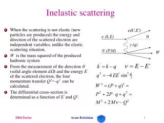
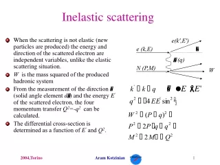
DIS kinematics ep collision proton in “∞” momentum frame No transverse momentum 0 ≤ x ≤ 1 x = fractional longitudinal momentum carried by the struck parton √s = ep cms energy Q2=-q2= 4-momentum transfer squared (or virtuality of the “photon”)
DIS kinematics Final electron energy ep collision Initial electron energy Q2=-q2=-(k-k’)2=2EeE’e(1+cosθe) EeE’e(1+cosθe) x =Q2/2P•q = EP 2Ee-E’e(1-cosθe) Initial proton energy Electron scattering angle Everything we need can be reconstructed from the measurement of E’eand θe. (in principle)
Deep Inelastic Scattering experiments HERA collider: H1 and ZEUS experiments 1992 – 2007 (will complete July 2, 2007) Fixed target DIS at SLAC, FNAL and CERN completed ~ 10-20 years ago
e-p Neutral Current (NC) cross-section: Has to do with long. photon. Only large at largest y We’ll come back to these Has to do with Z0 exchange: small for Q<<MZ d2σ 2πα2 = [Y+F2(x,Q2)-y2 FL(x,Q2)+Y-xF3(x,Q2)] dxdQ2 xQ4 y=Q2/xs 0 ≤ y ≤ 1 “inelasticity” Y±=1±(1-y) So for now: d2σ 2πα2 = Y+F2(x,Q2) dxdQ2 xQ4 quark charge 2 F2 = x∑(q + q) eq + Z-exchange quark and anti-quark distributions
IF, proton was made of 3 quarks each with 1/3 of proton’s momentum: no anti-quark! 2 F2 = x∑(q(x) + q(x)) eq q(x)=δ(x-1/3) F2 or with some smearing x 1/3 The partons are point-like and incoherent then Q2 shouldn’t matter. Bjorken scaling: F2 has no Q2 dependence. Let’s look at some data
Proton Structure Function F2 F2 Seems to be…. NOT
So what does this mean..? QCD, of course: q quarks radiate gluons q q gluons can produce qq pairs q gluons can radiate gluons!
Proton e’ ~1.6 fm (McAllister & Hofstadter ’56) γ*(Q2) e r Virtuality (4-momentum transfer) Q gives the distance scale r at which the proton is probed. r≈ hc/Q = 0.2fm/Q[GeV] CERN, FNAL fixed target DIS: rmin≈ 1/100 proton dia. HERA ep collider DIS: rmin≈ 1/1000 proton dia. HERA: Ee=27.5 GeV, EP=920 GeV
F2 Higher the resolution (i.e. higher the Q2) more branchings to lower x we “see”. So what do we expect F2 as a function of x at a fixed Q2to look like?
F2(x) Three quarks with 1/3 of total proton momentum each. x 1/3 F2(x) Three quarks with some momentum smearing. x 1/3 F2(x) The three quarks radiate partons at low x. x 1/3
Proton Structure Function F2 How this change with Q2 happens quantitatively described by the: Dokshitzer-Gribov-Lipatov-Altarelli-Parisi (DGLAP) equations
DGLAP equations are easy to “understand” intuitively First we have the four “splitting functions” z z z z 1-z 1-z 1-z 1-z Pab(z) : the probability that parton a will radiate a parton b with the fraction z of the original momentum carried by a.
Now DGLAP equations (schematically) convolution dqf(x,Q2) o o = αs[qf × Pqq + g × Pgq] d ln Q2 strong coupling constant Change of quark distribution q with Q2 is given by the probability that q and g radiate q. Same for gluons: dg(x,Q2) o o = αs[∑qf × Pqg + g × Pgg] d ln Q2
DGLAP fit (or QCD fit) extracts the parton distributions from measurements. (Lectures by Jeff Owens next week) Here’s a 1 min description: Step 1: parametrise the parton momentum desity f(x) at some Q2. e.g. uv(x) u-valence dv(x) d-valence g(x) gluon S(x) sum of all “sea” (i.e. non valence) quarks Step 2: find the parameters by fitting to DIS (and other) data using DGLAP equations to evolve f(x) in Q2. f(x)=p1xp2(1-x)p3(1+p4√x+p5x) “The orginal three quarks”
At x<<1/3, quarks and (antiquarks) are all “sea”. Since F2 = eq ∑x(q + q), xS is very much like F2 2 Sea PDF xS Fractional uncertainty x
Gluons, on the other hand, are determined from the scaling violations dF2/dlnQ2 via the DGLAP equations. Gluon PDF xg Uncertainties are larger. Scaling violations couple αs and gluon g Fit with αs also a free param. x
So far: F2 ~ ∑(q+q) ≈ S (sea quarks) measured directly in NC DIS Scaling violations dF2/dlnQ2 ~ αs•g Scaling violations gives gluons (times αs). DGLAP equations. What about valence quarks? ∑(q-q) = uv + dv can we determine them separately? Can we decouple αs and g ?
Return to Neutral Current (NC) cross-section: Now write out the e+p and e-p separately (keep ignoring FL for now..) Y±=1±(1-y) d2σ(e±p) 2πα2 = [Y+F2(x,Q2) Y-xF3(x,Q2)] ± dxdQ2 xQ4 xF3 = ∑(q(x,Q2)-q(x,Q2)) xBq ~The valence quarks! Bq = -2eqaqaeχZ+ 4vqaqveaeχZ Bq = -2eqaqaeχZ+ 4vqaqveaeχZ 2 2 1 Q2 χZ= ( ) Keeps xF3 small if Q<MZ 2 sin2θW MZ+Q2
Return to Neutral Current (NC) cross-section: Now write out the e+p and e-p separately (keep ignoring FL for now..) Y±=1±(1-y) d2σ(e±p) 2πα2 = [Y+F2(x,Q2) Y-xF3(x,Q2)] ± dxdQ2 xQ4 xF3 = ∑(q(x,Q2)-q(x,Q2)) xBq ~The valence quarks! Bq = -2eqaqaeχZ+ 4vqaqveaeχZ Bq = -2eqaqaeχZ+ 4vqaqveaeχZ 2 2 γ-Z interference Z-exchange eq: electric charge of a quark aqvq: axial-vector and vector couplings of a quark aeve: axial-vector and vector couplings of an electron
Return to Neutral Current (NC) cross-section: Now write out the e+p and e-p separately (keep ignoring FL for now..) Y±=1±(1-y) d2σ(e±p) 2πα2 = [Y+F2(x,Q2) Y-xF3(x,Q2)] ± dxdQ2 xQ4 xF3 = ∑(q(x,Q2)-q(x,Q2)) xBq ~The valence quarks! Let’s look at the “reduced NC cross-section” σNC± = F2(x,Q2) (Y-/Y+)•xF3(x,Q2) ± Note the change of sign from e+p to e-p
Reduced Neutral Current Cross-section σNC± x Measurements are at relatively high x
Charged Current Cross-Sections 2 2 dσCC(e±p) GF MW = [ ]2σCC± dxdQ2 2πx MW+Q2 2 Skip a few steps…. σCC+ = x [u + c + (1 - y)2(d + s)] ~ d σCC- = x [u + c + (1 – y)2(d + s)] ~ u charm
Reduced Charged-Current Cross-Section σCC± σCC+ ~ d σCC- ~ u x Now let’s look at the valence quarks from the QCD fits
Valence PDFs xf x The momenta from valence quarks are producing gluons and sea quarks at low x
Jet production in DIS (HERA) σjet ~ αs•f(x) Sensitive to αs Sensitive to gluon ~10-3 < x < ~10-2 Sensitive to quarks ~10-2 < x < ~10-1 complementary to gluon from F2 Same range as NC and CC
Jet measurements in Breit frame No ET in Breit Frame Jet production cross-section used in QCD fit
Gluon distributions x x Using only HERA (ZEUS) data including NC,CC and jets Using HERA (ZEUS) F2 data and FNAL, CERN fixed tgt
Proton Structure Function F2 F2 Now we understand what is happening here.
Some remarks about DGLAP equations: The “incoherence” of the original parton model is preserved. i.e. a parton doesn’t know anything about its neighbor. never happens The “process independent” partons also survive. But now parton densities must be “evolved” in Q2. What does this mean?
A parton at x at Q2is a source of partons at x’ < x at Q’2 > Q2. In fact, any parton at x > x’ at Q2is a source. unknown Q’2 known To know the parton density at x’, Q’2 it’s necessary (and sufficient) to know the parton density in the range: x’ ≤ x ≤ 1 at some lower Q2. Q2 measured 1 x’ x If you know the partons in range x’ ≤ x ≤ 1 at some Q2, then you know the partons in the range x’ ≤ x ≤ 1 for all Q’2 > Q2. What does this mean for the LHC?
Tevatron jets “known” HERA DIS Fixed target DIS ~safe Q2
LHC (or hadron-hadron) parton kinematics rapidity: 1 E+PZ y= ln( ) 2 E-PZ pseudo-rapidity: η=-ln tan(θ/2) 2 4 angle wrt beam parton1(x1) + parton2(x2) State with mass M x1= (M/√s) exp (y) x2= (M/√s) exp (-y)
σ(ppW,Z+X) ~ q,q(x1,MW,Z) × q,q(x2,MW,Z) × σ(qqW,Z) 2 2 So if I want to predict Z or W production cross-section at LHC at some rapidity y, say, -4: need and 2 4 2 2 q,q(x1=10-4,Q2=MW,Z) q,q(x2=0.3,Q2=MW,Z)
Evolving PDFs up to MW,Z scale xf(x) xg(x) “evolved” xS(x) “measured” “measured” xg(x) xS(x)
Examples of predictions for LHC using partons from DIS Jet production at LHC Z production at LHC Uncertainty ~5% σ(arb. scale) -6 η 6 A. Cooper-Sarkar (HERA-LHC workshop 2007)
Final remarks I • We’ve just gone through an informal tour of QCD-improved parton model and its application to data from ep Deep Inelastic Scattering. • Some health warnings: • Most of what I talked about is a leading-order picture. In practice, most things are done at least to next-to-leading order. At NLO, the interpretation of the results are not as straight-forward. • Many people worry about whether we are not missing something fundamentally with the picture of DGLAP equations. • Much of the data are at very low x: DGLAP is a lnQ2 approximation. Why aren’t ln(1/x) terms important…or are they? BFKL equations. • The density of the partons, especially that of the gluons is getting very high. When and where should we worry about “shadowing”, “gluon recombination” etc. • The idea of incoherence of partons may be breaking down in some kinematic regions: phenomenon of “hard diffraction” is difficult to understand in terms of partons without correlations to each other.
Final remarks II • There are many other DIS physics topics I did not cover here. • Electoweak physics • Heavy quark production • Diffraction, Vector Meson production, low Q2 physics • Beyond the SM searches. • Polarized DIS • … • I hope I have refreshed your memory about some familiar DIS physics, and got you ready for the rest of the school. • Thanks to the organizers for their kind invitation. Thanks to Claire Gwenlan for preparing some of the plots animation for me. • You can find the animated gifs in: • http://www.hep.anl.gov/ryoshida/animated_proton.htm
Longitudinal cross-section FL=(Q2/4π2α) σL
QCD predicts a relationship between scaling violations and FL through the gluon density. increasing y
You can determine FL from a NLO DGLAP fit to NC cross-section. Indeed, we also only determine F2 the same way, in principle: We measure this only x
HERA measurement of FL on-going now Normally 920 GeV C. Diaconu: DIS 07 conference April 07