Expectations and our IS-LM model
220 likes | 492 Vues
Expectations and our IS-LM model. In this lecture we will examine how expectations about the future will impact investment and consumption today. We will introduce some new ways of thinking about how people make the choice about how much to consume today.

Expectations and our IS-LM model
E N D
Presentation Transcript
Expectations and our IS-LM model • In this lecture we will examine how expectations about the future will impact investment and consumption today. • We will introduce some new ways of thinking about how people make the choice about how much to consume today. • We will then return to our IS-LM framework. We will show how expectations about the future can affect output and interest rates through changes in consumption and investment decisions.
New investment function • Last week we showed that the share value of a firm must be equal to the present value of the stream of future dividends of the firm. Pt = det+1/(1+it) + det+2/(1+iet+1)(1+it) + … • But the dividends can only come out of profits, either profits today or delayed past profits that were reinvested in the firm. • Any profit that is reinvested into the firm must earn at least an it return on the profit, or the share price will drop.
Investment function • In this case we can also think of share price as: Pt = Profitset+1/(1+it) + Profitset+2/(1+iet+1)(1+it) + … • The share price is the present value of the expected stream of future profits. • In the simple case where expected profits are constant and the expected interest rate was constant, this simplified to: Pt = Profitse/ie • The higher is Pt the greater is the incentive to invest.
Investment function • Our investment function can be imagined to be: It = I(Profitse/ie) • The book’s derivation uses similar logic in real values instead of nominal values which we are using here to derive: It = I(Real Profitse/(re+δ)) • Where δ is the rate of depreciation of capital over time, ie. wearing out. • Since i and r are related through the Fisher equation, the forms of these two functions will be similar.
Understanding consumption • Our consumption decision has been modelled as Ct = c0 + c1 Yt • So we have assumed that the amount of resources consumed today is a linear function of today’s income. • How reasonable an assumption is this? • The aggregate consumption of an economy must be nothing more than the sum of the individual consumption choices of all the households in an economy.
Household consumption • Can we learn anything about the behaviour of aggregate consumption by understanding how individual households make consumption choices? • How do individuals/households plan their consumption? • Fact 1: Consumption choices are constrained by people’s incomes. • Households can borrow money to pay for consumption, but any borrowings must be matched by a later repayment. Borrowings can not increase wealth of a household.
Time profile of income • Fact 2: Over a lifetime, people generally make little money in their 20s, income increases in 30s and 40s, peaks in their mid 50s and they earn nothing after 65. • Consumption could match income in every year, but then you would live poorly while young and starve to death after 65.
Time profile of consumption • Most people would prefer a flatter “time profile” of consumption. • This could be achieved by borrowing while young, repaying the borrowings and accumulating some savings while middle-aged and then living off savings when retired.
Time profile of net assets • To do this households would accumulate debt while young (mortgages etc), repay the debt and accumulate savings in middle aged and then live off savings while old. Perhaps leaving some savings to children.
Human wealth • What matters then for the time profile of a household’s consumption are the total assets of the household. • Where assets here mean financial wealth like savings accounts, housing wealth like mortgages and human wealth which is the present value of after-tax future income. • What is my human wealth? Ht = (1-t)Yt+1e /(1+it) + (1-t)Yt+2e /(1+it+1e ) + … • Where t is the share of your income taken by the government. • My human wealth is discounted present value.
Household consumption plan • My consumption decision is a matter of choosing how to allocate my household’s resources to consumption over time. • Your consumption plan can change for many reasons. • A change is likely to affect consumption in every year, and not just this year’s consumption. • One of the household may need expensive medical treatment, so you have to pay for the treatment out of wealth and lower consumption at all times.
Changes in plans • An expected change in the future will likely have an impact on consumption today. • If I know that I will be wealthier in the future (a rich aunt puts the family in her will), I may choose to increase consumption today. • A change that is permanent will have a larger impact than a temporary change. • A tax cut of $1,000 for this year only will increase consumption slightly as it only raises household wealth by $1,000. • A permanent tax increase of $1,000 raises household wealth by the discounted present value of $1,000 for the number of working years remaining for household.
Temporary versus permanent • A permanent tax cut raises current income by $1,000 and raises human wealth by: $1,000 /(1+it) + $1,000 /(1+it+1e ) + … • Which for young households will be close to $1,000/i. • So for a temporary tax cut, we might not expect consumption to rise very much as households will spread the $1,000 in new wealth over their whole consumption plan. • But for a permanent tax cut of $1,000, households can raise their consumption in each year by almost $1,000 and still remain within their budgets.
Temporary versus permanent • In our model of aggregate consumption, we had: Ct = c0 + c1 Yt • For a temporary tax cut, c1 would be low as households do not consume much of the tax cut today. • For a permanent tax cut, c1 would be high as households consume almost all of the tax cut today. • This means that we can not represent aggregate consumption in this linear form.
New consumption function • We have to adopt a new form Ct = C(Yt , Wt ) • Where Wt is our household wealth, which will be the sum of our financial and housing assets, At , plus our human wealth, Ht . Wt = At + Ht • A simple example might be something like: Ct = c0 + c1 Yt + c2 Wt • A temporary tax cut of $1 raises consumption by c1 but a permanent tax cut raises consumption by close to c1 + c2/i.
Back to our IS-LM model • We have adjusted our IS equation to allow for expectations of the future. • Our new consumption function Ct = C(Yt, Tt, Wt ) • Allows for the fact that consumption will be affected by changes in household wealth. • Our new investment function It = I(Real Profitse/(re+δ)) • Allows for the fact that investment depends on expectations of future profits and interest rates.
Present versus future • One way to analyse effects is to think of changes that affect variables today and/or variables tomorrow. • We have already been thinking this way when we think of temporary versus permanent tax cuts. • We can arbitrarily divide our variables into present income (Y) and future income (Ye), present taxes (T) and future taxes (Te), present real interest rates (r) and future real interest rates (re).
Deriving a new IS equation • Wealth (and so also consumption) will be affected by Ye, re and Te. The effect of Ye and Te on wealth is obvious, but what about re? • Real assets of a household change from year to year by: At = (1 + rt-1) [At-1 + Yt-1 – Ct-1] • We assume that left-over real assets are invested. • So a higher re will increase the wealth of people who has positive assets and reduce the wealth of people with negative assets.
Deriving a new IS equation • A higher re will also reduce human wealth. The net result on net wealth is ambiguous, so we ignore the effect of re on wealth. • A higher re will have a negative effect on investment through the investment function. We assume future profits (and so also investment) will be affected positively by future income and negatively by future taxes.
Deriving a new IS equation • Our new IS equation becomes: Y = C(Y, T, W(Ye, Te)) + I(Profits(Ye, Te), r, re) + G • Avoiding the book’s ugly notation, let’s just use IS for the right-hand side. Y = IS(Y, T, r, Ye, Te, re, G) (+, -, -, +, -, -, +) • Where IS = A + G in the book’s notation and the +/- are the relationships between and increase in the independent variable and Y.
Deriving a new IS equation • What is important to remember here are the channels through which the right-hand side variables affect the IS equation, ie. an increase in Ye raises C because wealth rises and raises I because future profits rise. • Example: Imagine the government increases G without raising taxes today- issuing debt instead. But people know that this new debt will have to be paid off with future taxes, so Te rises.
The increase in G will shift the IS curve to the right. This would be where our analysis would end without expectations. However now we know that Te rises, so future wealth falls and present consumption drops. The net effect on the IS curve is ambiguous. Deficit spending Example: deficit spending r Te G IS Y