The Smoothed Analysis of Algorithms
470 likes | 1.48k Vues
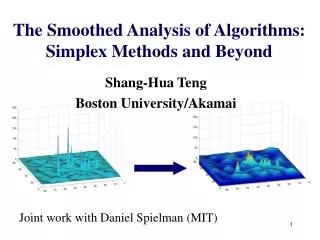
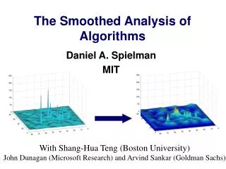
The Smoothed Analysis of Algorithms. Daniel A. Spielman MIT. With Shang-Hua Teng (Boston University) John Dunagan (Microsoft Research) and Arvind Sankar (Goldman Sachs). Outline. Why?. What?. The Simplex Method. Gaussian Elimination. Other Problems. Conclusion. Problem:

The Smoothed Analysis of Algorithms
E N D
Presentation Transcript
The Smoothed Analysis of Algorithms Daniel A. Spielman MIT With Shang-Hua Teng (Boston University) John Dunagan (Microsoft Research) and Arvind Sankar (Goldman Sachs)
Outline Why? What? The Simplex Method Gaussian Elimination Other Problems Conclusion
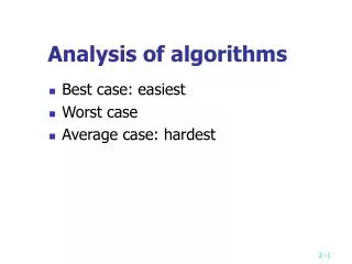
Problem: Heuristics that work in practice, with no sound theoretical explanation Exponential worst-case complexity, but works in practice Polynomial worst-case complexity, but much faster in practice Heuristic speeds up code, with poor results in worst-case
Attempted resolution: Average-case analysis Measure expected performance on random inputs
Random is not typical
Critique of Average-case Analysis Random objects have very special properties with exponentially high probability Actual inputs might not look random.
Smoothed Analysis: a hybrid of worst and average case worst case average case
Smoothed Analysis: a hybrid of worst and average case is Gaussian of stand dev worst case average case smoothed complexity
Smoothed Complexity Interpolates between worst and average case Considers neighborhood of every input If low, all bad inputs are unstable
Complexity Landscape worst case run time average case input space
Smoothed Complexity Landscape(convolved with Gaussian) run time smoothed complexity input space
Classical Example: Simplex Method for Linear Programming max s.t. Worst-Case: exponential Average-Case: polynomial Widely used in practice
The Diet Problem Min s.t.
Classical Example: Simplex Method for Linear Programming max s.t. Worst-Case: exponential Average-Case: polynomial Widely used in practice
The Simplex Method opt start
max s.t. max s.t. Smoothed Analysis of Simplex Method G is Gaussian Theorem: For all A, b, c, simplex method takes expected time polynomialin
Analysis of Simplex Method Using Shadow-Vertex Pivot Rule
Shadow vertex pivot rule start objective
Polar Form of Linear Programming c max cÎ ConvexHull(a1, a2, ..., am)
Count pairs in different facets [ ] Different Facets < c/N Pr So, expect c Facets
Angle Distance
max s.t. max s.t. Smoothed Analysis of Simplex Method G is Gaussian Theorem: For all A, b, c, simplex method takes expected time polynomialin
Interior Point Methods for Linear Programming Analysis Method #Iterations Observation Worst-Case, upper Worst-Case, lower Average-Case Smoothed, upper ( ) [Dunagan-S-Teng], [S-Teng] Conjecture
Gaussian Elimination for Ax = b >> A = randn(2) A = -0.4326 0.1253 -1.6656 0.2877 >> b = randn(2,1) b = -1.1465 1.1909 >> x = A \ b x = -5.6821 -28.7583 >> norm(A*x - b) ans = 8.0059e-016
Gaussian Elimination for Ax = b >> A = 2*eye(70) - tril(ones(70)); >> A(:,70) = 1; >> b = randn(70,1); >> x = A \ b; >> norm(A*x - b) ans = 3.5340e+004 Failed! Perturb A >> Ap = A + randn(70) / 10^9; >> x = Ap \ b; >> norm(Ap*x - b) ans = 5.8950e-015
>> A = 2*eye(70) - tril(ones(70)); >> A(:,70) = 1; >> b = randn(70,1); >> x = A \ b; >> norm(A*x - b) ans = 3.5340e+004 Failed! Perturb A >> Ap = A + randn(70) / 10^9; >> x = Ap \ b; >> norm(Ap*x - b) ans = 5.8950e-015 >> norm(A*x - b) ans = 3.6802e-008 Solved original too! Gaussian Elimination for Ax = b
>> A = 2*eye(70) - tril(ones(70)); >> A(:,70) = 1; >> b = randn(70,1); >> x = A \ b; >> norm(A*x - b) ans = 3.5340e+004 Failed! Perturb A >> Ap = A + randn(70) / 10^9; >> x = Ap \ b; >> norm(Ap*x - b) ans = 5.8950e-015 >> norm(A*x - b) ans = 3.6802e-008 Solved original too! Gaussian Elimination for Ax = b
>> A = 2*eye(70) - tril(ones(70)); >> A(:,70) = 1; >> b = randn(70,1); >> x = A \ b; >> norm(A*x - b) ans = 3.5340e+004 Failed! Perturb A >> Ap = A + randn(70) / 10^9; >> x = Ap \ b; >> norm(Ap*x - b) ans = 5.8950e-015 >> norm(A*x - b) ans = 3.6802e-008 Solved original too! Gaussian Elimination for Ax = b
Gaussian Elimination with Partial Pivoting Fast heuristic for maintaining precision, by trying to keep entries small
Gaussian Elimination with Partial Pivoting Fast heuristic for maintaining precision, by trying to keep entries small Pivot not just on zeros, but to move up entry of largest magnitude
Gaussian Elimination with Partial Pivoting “Gaussian elimination with partial pivoting is utterly stable in practice. In fifty years of computing, no matrix problems that excite an explosive instability are know to have arisen under natural circumstances … Matrices with large growth factors are vanishingly rare in applications.” Nick Trefethen
Gaussian Elimination with Partial Pivoting “Gaussian elimination with partial pivoting is utterly stable in practice. In fifty years of computing, no matrix problems that excite an explosive instability are know to have arisen under natural circumstances … Matrices with large growth factors are vanishingly rare in applications.” Nick Trefethen Theorem: [Sankar-S-Teng]
Mesh Generation Parallel complexity of Ruppert’s Delaunay refinement is O( (log n/s)2) Spielman-Teng-Üngör
Other Smoothed Analyses Perceptron[Blum-Dunagan] Quicksort[Banderier-Beier-Mehlhorn] Parallel connectivity in digraphs [Frieze-Flaxman] Complex Gaussian Elimination [Yeung]Smoothed analysis of K(A) [Wschebor] On smoothed analysis in dense graphs and formulas [Krivelevich-Sudakov-Tetali]Smoothed Number of Extreme Points under Uniform Noise [Damerow-Sohler] Typical Properties of Winners and Losers in Discrete Optimization [Beier-Vöcking] Multi-Level Feedback scheduling [Becchetti-Leonardi-Marchetti-Shäfer-Vredeveld] Smoothed motion complexity [Damerow, Meyer auf der Heide, Räcke, Scheideler, Sohler]
Future Smoothed Analyses Multilevel graph partitioning Smoothed Analysis of Chaco and Metis Differential Evolution and other optimization heuristics Computing Nash Equilibria
Future Smoothed Analyses Perturb less! Preserve zeros Preserve magnitudes of numbers Property-preserving perturbations More Discrete smoothed analyses New algorithms For more, see the Smoothed Analysis Homepage