Types of search
490 likes | 512 Vues
Discusses the three types of search in CS: for stored data, for a path to a goal, and for solutions using examples. Detailed explanation of uninformed and informed search methods with illustrative examples.

Types of search
E N D
Presentation Transcript
Types of search In CS, there are at least three overlapping meanings of “search”: • Search for stored data (conventional search). This assumes an explicitly described collection of information (for example, a DB), and the goal is to search for a specified item. Examples: binary search, graph search algorithms studied in CS 253. • Search for a path to a specified goal (AI search). This suggests a search space which is not explicitly defined, except for the initial state, the goal state and the set of operators to move from one state to another. The goal is to find a path from the initial state to the goal state by examining only a small portion of the search space. Examples to be discussed: depth-first search, A* search, and more. • Search for solutions. This is a more general type of a search compared to the search for a path to a goal. The idea is to efficiently find a solution to a problem among a large number of candidate solutions comprising the search space. It is assumed that at least some (but not all) candidate solutions are known in advance. The problem is how to select a subset of a presumably large set of candidate solutions to evaluate. Examples to be discussed: hill-climbing, simulated annealing, genetic algorithms.
Search for a path in a conceptually specified graph. Consider a goal-based agent capable of formulating a search problem by: • providing a description of the current problem state, • providing a description of its own actions that can transform one problem state into another one, • providing a description of the goal state where a desired goal holds. The solution of such a problem consists of finding a path from the current state to the goal state. The problem space can be huge, which is why the agent must know how to efficiently search it and evaluate solutions.To define how “good” the solution is, a path cost function can be assigned to a path. Different solutions of the same problem can be compared by means of the corresponding path cost functions. We shall discuss two types of searches: • Uninformed search (no problem-specific information is available to direct the search). We shall use the Missionaries and Cannibals (M&C) problem to illustrate uninformed search. • Informed search (there is a problem-specific information helping the agent through the search process). We shall use the 5-puzzle problem (a downsized version of the 8-puzzle problem) to illustrate informed search.
Uninformed search example: the Missionaries and Cannibals problem. The search problem is defined as follows: • Description of the current state: a sequence of six numbers, representing the number of missionaries, cannibals and boats on each bank of the river. Assuming 3 missionaries, 3 cannibals and one boat, the initial state is (setf start '(3 3 1 0 0 0)) • Description of possible actions (or operators): take either one missionary, one cannibal, two missionaries, two cannibals, or one of each across the river in the boat, i.e. (setf list-of-actions '((1 0 1) (0 1 1) (2 0 1) (0 2 1) (1 1 1))) • Description of the goal state, i.e. (setf finish '(0 0 0 3 3 1)) Note that some world states are illegal (the number of cannibals must always be less or equal to the number of missionaries on each side of the river. Therefore, we must impose certain constraints on the search to avoid illegal states. We also must guarantee that search will not fall in a loop (some actions may “undo” the result of a previous action).
3,3,1,0,0,0 3,1,1,0,2,0 3,1,0,0,2,1 3,2,0,0,1,1 3,2,1,0,1,0 3,0,0,0,3,1 3,0,1,0,3,0 2,2,0,1,1,1 2,3,0,1,0,1 1,3,0,2,0,1 2,2,1,1,1,0 2,0,1,1,3,0 2,1,1,1,2,0 2,1,0,1,2,1 2,3,1,1,0,0 1,3,1,2,0,0 1,1,1,2,2,0 1,2,1,2,1,0 1,0,1,2,3,0 2,0,0,1,3,1 1,1,0,2,2,1 1,2,0,2,1,1 0,3,0,3,0,1 0,2,1,3,1,0 0,1,1,3,2,0 0,1,0,3,2,1 0,3,1,3,0,0 3,3,0,0,0,1 0,2,0,3,1,1 0,0,0,3,3,1 The problem space for the M&C problem Problem space is a complete description of the domain. It can be huge, which is why it is only procedurally defined. Here is the problem space for the M&C problem.
Search (or solution) space is a part of the problem space which is actually examined 3,3,1,0,0,0 [1,1,1] [0,2,1] [0,1,1] 2,2,0,1,1,1 3,2,0,0,1,1 3,1,0,0,2,1 [1,0,1] [0,1,1] Dead end 3,2,1,0,1,0 3,2,1,0,1,0 [1,0,1] [0,1,1] [0,2,1] [0,2,1] 3,0,0,0,3,1 3,1,0,0,2,1 3,0,0,0,3,1 2,2,0,1,1,1 Dead end Dead end ... ...
Depth-first search: always expand the path to one of the nodes at the deepest level of the search tree Each path is a list of states on that path, where each state is a list of six elements (m1 c1 b1 m2 c2 b2). Initially, the only path contains only the start state, i.e. ((3 3 1 0 0 0)). (defun depth-first (start finish &optional (queue (list (list start)))) (cond ((endp queue) nil) ((equal finish (first (first queue))) (reverse (first queue))) (t (depth-first start finish (append (extend (first queue)) (rest queue)))))) (defun extend (path) (setf extensions (get-extensions path)) (mapcar #'(lambda (new-node) (cons new-node path)) (filter-extensions extensions path)))
Breadth-first search: always expand all nodes at a given level, before expanding any node at the next level (defun breadth-first (start finish &optional (queue (list (list start)))) (cond ((endp queue) nil) ((equal finish (first (first queue))) (reverse (first queue))) (t (breadth-first start finish (append (rest queue) (extend (first queue))))))) (defun extend (path) (setf extensions (get-extensions path)) (mapcar #'(lambda (new-node) (cons new-node path)) (filter-extensions extensions path)))
Depth-first vs breadth-first search Depth-firstsearch 1. Space complexity: O(bd), where b is the branching factor, and d is the depth of the search. 2. Time complexity: O(b^d). 3. Not guaranteed to find the shortest path (not optimal). 4. Not guaranteed to find a solution (not complete) 5. Polynomial space complexity makes it applicable for non-toy problems. Breadth-first search 1. Space complexity: O(b^d) 2. Time complexity: O(b^d). 3. Guaranteed to find the shortest path (optimal). 4. Guaranteed to find a solution (complete). 5. Exponential space complexity makes it impractical even for toy problems.
Other uninformed search strategies. • Depth-limited is the same as depth-first search, but a limit on how deep into a given path the search can go, is imposed. In M&C example, we avoided unlimited depth by checking for cycles. If the depth level is appropriately chosen, depth-limited search is complete, but not optimal. Its time and space complexity are the same as for the depth-first search, i.e. O(b^d) and O(bd), respectively. • Iterative deepening is a combination of breadth-first and depth-first searches, where the best depth limit is determined by trying all possible depth limits. Its space complexity is O(bd), which makes it practical for large spaces where loops are possible, and therefore the depth-first search cannot be successful. It is optimal, i.e. guaranteed to find the shortest path. • Bi-directional search is initiated simultaneously from the initial state and goal state in a hope that the two paths will eventually meet. It is complete and optimal, but its time and space efficiencies are exponential, i.e. O(b^(d/2)).
Informed search strategies: best-first “greedy” search Best-first search always expends the node that is believed to be the closest to the goal state. This is defined by means of the selected evaluation function. Example: consider the following graph whose nodes are represented by means of their property lists: (setf (get 's 'neighbors) '(a d) (get 'a 'neighbors) '(s b d) (get 'b 'neighbors) '(a c e) (get 'c 'neighbors) '(b) (get 'd 'neighbors) '(s a e) (get 'e 'neighbors) '(b d f) (get 'f 'neighbors) '(e)) (setf (get 's 'coordinates) '(0 3) (get 'a 'coordinates) '(4 6) (get 'b 'coordinates) '(7 6) (get 'c 'coordinates) '(11 6) (get 'd 'coordinates) '(3 0) (get 'e 'coordinates) '(6 0) (get 'f 'coordinates) '(11 3))
To see the description of a node, we can say: * (describe 'a) ........ Property: COORDINATES, Value: (4 6) Property: NEIGHBORS, Value: (S B D) To find how close a given node is to the goal, we can use the formula computing the straight line distance between the two nodes: (defun distance (node-1 node-2) (let ((coordinates-1 (get node-1 'coordinates)) (coordinates-2 (get node-2 'coordinates))) (sqrt (+ (expt (- (first coordinates-1) (first coordinates-2)) 2) (expt (- (second coordinates-1) (second coordinates-2)) 2)))))
Given two partial paths, whose final node is closest to the goal, can be defined by means of the following closerp predicate: (defun closerp (path-1 path-2 finish) (< (distance (first path-1) finish) (distance (first path-2) finish))) The best-first search now means “expand the path believed to be the closest to the goal”, i.e. (defun best-first (start finish &optional (queue (list (list start)))) (cond ((endp queue) nil) ((equal finish (first (first queue))) (reverse (first queue))) (t (best-first start finish (sort (append (extend (first queue)) (rest queue)) #'(lambda (p1 p2) (closerp p1 p2 finish))))))) (defun extend (path) (mapcar #'(lambda (new-node) (cons new-node path)) (remove-if #'(lambda (neighbor) (member neighbor path)) (get (first path) 'neighbors))))
A* search: a combination of the best-first greedysearch and uniform-cost search • Uniform-cost search takes into account the path cost, and expands always the lowest cost node. Assume that this path cost is g(n). • Best-first search expands the node which is believed to be the closest to the goal. Assume that the estimated cost to reach the goal from this node is h(n). A* search always expands the node with the minimum f(n), where f(n) = g(n) + h(n). We assume here that f(n) never decreases, i.e. f(n) is a monotonic function. Under this condition, A* search is both optimal and complete. A* is hard to implement because any time a shorter path between the start node and any node is found, A* must update cost of paths going through that node.
3 2 1 2 3 1 5 0 4 5 0 The 5-puzzle problem (a downsized version of the 8-puzzle problem) Here is an example of the 5-puzzle problem: Consider the following representation: • Initial state description: (4 3 2 1 5 0) • Possible moves: move the empty “0” tile up, down, left or right depending on its current position. • Goal state description: (1 2 3 4 5 0) The problem space contains 6! = 720 different states (for the 8-puzzle, it is 9! = 362,880 different states). However, assuming the branching factor of 2 and a length of a typical solution of about 15, exhaustive search would generate about 2^15 = 32,768 states (for the 8-puzzle, these numbers are: branching factor 3, typical solution is about 20 steps, or 3^20 = 3.5 * 10^9 states).
Solving the 5-puzzle problem We shall compare the following searches for solving the 5-puzzle problem (some of this comparison will be done by you as part of homework 2): • Breadth-first search, which is a special case of uniform-cost search where g(n) = depth(n) (as it guarantees to find the shortest path given enough time and space). • Best-first search with 2 heuristic functions : • Number of tiles in place (or number of tiles out of place). • Manhattan distance. It computes the distance of each tile from its final place, i.e. the distance between the tile’s current and final position in the horizontal direction plus the distance in the vertical direction. • Depth-limited search (similar to depth-first, but the maximum path length is limited to prevent infinite paths). Notes: 1. The search space for this type of puzzles is known to be not fully interconnected, i.e. it is not possible to get from one state to any other state. Initial states must be carefully selected so that the final state is reachable from the initial state. 2. Best-first search using an admissible heuristic is known to be equivalent to A* (exponential, but is both optimal and complete). Our heuristics here are not optimal because we do not account for g(n), i.e. how we got to the current state.
Search for solutions (iterative improvement): hill-climbing search If the current state contains all the information needed to solve the problem, then we try the best modification possible to transform the current state into the goal state. (defun hill-climb (start finish &optional (queue (list (list start)))) (cond ((endp queue) nil) ((equal finish (first (first queue))) (reverse (first queue))) (t (hill-climb start finish (append (sort (extend (first queue)) #'(lambda (p1 p2) (closerp p1 p2 finish))) (rest queue))))))
Best applications for a hill-climbing search are those where initial state contains all the information needed for finding a solution. Example: N-queens problem, where initially all queens are on the board, one queen per column (the problem is completely defined), so-called complete set formulation. The successors are all possible states generated by moving a single queen to another square in the same column (up or down move). Queens are moved around until no queen attacks any other. Notice that the initial state is not fixed. We may start with any configuration of N queens, but there is no guarantee that a solution exists for that particular configuration. If a dead end is encountered, “forget” everything done so far and re-start from a different initial configuration. No need to store the search tree; only the current state is relevant at each time, because it completely defines the problem.
Best-first search vs hill-climbing search Best-first search 1. Space complexity: O(b^d), because the whole search tree is stored in the memory. 2. Time complexity: O(b^d). A good heuristic function can substantially improve this worst case. 3. Greedy search: not complete, not optimal. A* search: complete and optimal if the estimated cost for the cheapest solution through n, f(n), is a monotonic function. Hill-climbing search 1. Space complexity: O(1), because only a single state is maintained in the memory. 2. Time complexity: O(b^d). 3. Not complete, because of the local maxima phenomena (the goal state is not reached, but no state is better that the current state). Possible improvement: simulated annealing, which allows the algorithm to backtrack from the local maxima in an attempt to find a better continuation. 4. Not optimal.
Variations of hill-climbing: beam search and stochastic beam search Beam search stores only width best partial paths in the queue: (defun beam (start finish width &optional (queue (list (list start)))) (setf queue (butlast queue (max (- (length queue) width) 0))) ;;; trim partial paths from the end to (cond ((endp queue) nil) ;;; keep only width best ones. ((equal finish (first (first queue))) (reverse (first queue))) (t (beam start finish width (sort (apply #'append (mapcar #'extend queue)) ;;; extend all partial paths and sort #'(lambda (p1 p2) (closerp p1 p2 finish))))))) ;;; by distance to the goal Stochastic beam search instead of width best partial paths chooses width partial paths at random, but the probability of being chosen depends on utility function associated with partial paths.
Genetic Algorithms The Genetic Algorithm (GA) is a modification of stochastic beam search, where successor states are generated by combining two parent states, not by extending a single state. The underlying idea is to evolve a population of candidate solutions to a given problem using operators inspired by natural genetic variation and selection. Note that evolution is not a purposive or directed process; in biology, it seems to boil down to different individuals competing for resources in the environment. Some are better than others, and they are more likely to survive and propagate their genetic material. In very simplistic terms, the GA works as follows: • Identify initial set (population) of candidate solutions to the problem at hand. • Define a function to evaluate how “good” a candidate solution is. • Select pairs of candidate solutions to produce their offspring. • Replace “old” candidate solutions with these offspring, and repeat this process a specified number of times (generations).
Genetic algorithms: basic terminology [https://www.tutorialspoint.com/genetic_algorithms/genetic_algorithms_fundamentals.htm] Population: a subset of all the possible (encoded as string of bits) solutions to the given problem (analogous to the population for human beings except that instead of human beings, we have candidate solutions representing human beings). Example: 00110101, 01110001, 11000011, etc. Chromosome: a candidate solution encoded as a string of bits. Example: 00110101. Gene: one element position of a chromosome (a single bit, or short blocks of adjacent bits in more complex versions). Allele: the actual value of the gene (0 in the first gene in the chromosome example). Genotype: the population in the computation space, where solutions are represented in a way which can be easily understood and manipulated by a program. Phenotype: the population in the real world solution space, where solutions are represented in real world situations. Encoding and Decoding: a process of transforming from the phenotype to genotype, and a process of transforming a solution from the genotype to the phenotype, respectively.
GA operators Simplest genetic algorithms involve the following three operators: Selection: this operator selects chromosomes from the population according to their fitness for reproduction. Some GAs use a simple function of the fitness measure called fitness-proportionate selection. Other implementations use a model in which certain randomly selected individuals in a subgroup compete and the fittest is selected. This is called tournament selection. Crossover: this operator randomly chooses a point and exchanges the subsequences before and after that point between two chromosomes to create two offspring. For example, consider chromosomes 1100 0001 and 0001 1111. If they crossover after their forth point, the two offspring will be 1100 1111 and 0001 0001. Mutation: this operator randomly converts some of the bits in a chromosome. For example, if mutation occurs at the second bit in chromosome 11000001, the result is 10000001.
A simple genetic algorithm The outline of a simple genetic algorithm is the following: • Start with the randomly generated population of “n” j-bits chromosomes. • Evaluate the fitness of each chromosome. • Repeat the following steps until n offspring have been created: • Select a pair of parent chromosomes from the current population based on their fitness. • With the probability pc, called the crossover rate, crossover the pair at a randomly chosen point to form two offspring. If no crossover occurs, the two offspring are exact copies of their respective parents. • Mutate the two offspring at each gene with probability pm, called the mutation rate, and place the resulting chromosomes in the new population. If n is odd, one member of the new population is discarded at random. • Replace the current population with the new population. • Go to step 2. Each iteration of this process is called a generation. Typically, a GA produces between 50 to 500 generations in one run of the algorithm. Since randomness plays a large role in this process, the results of two runs are different, but each run at the end produces one or more highly fit chromosomes.
Example Assume the following: • length of each chromosome = 8, • fitness function f(x) = the number of ones in the bit string, • population size n = 4, • crossover rate pc = 0.7, • mutation rate pm = 0.001 The initial, randomly generated, population is the following: Chromosome label Chromosome string Fitness A 00000110 2 B 11101110 6 C 00100000 1 D 00110100 3
D B C A Example (cont.): step 3a We will use a fitness-proportionate selection, where the number of times an individual is selected for reproduction is equal to its fitness divided by the average of the fitnesses in the population, which is (2 + 6 + 1 + 3) / 4 • For chromosome A, this number is 2 / 3 = 0.667 • For chromosome B, this number is 6 / 3 = 2 • For chromosome C, this number is 1 / 3 = 0.333 • For chromosome D, this number is 3 / 3 = 1 (0.667 + 2 + 0.333 + 1 = 4) To implement this selection method, we can use “roulette-wheel sampling”, which gives each individual a slice of a circular roulette wheel equal to the individual’s fitness, i.e. Assume that the roulette wheel is spun, and the ball comes to rest on some slice; the individual corresponding to that slice is selected for reproduction. Because n = 4, the roulette wheel will be spun four times. Let the first two spins choose B and D to be parents, and the second two spins choose B and C to be parents.
Example (cont.): steps 3b and 3c Step 3bApply the crossover operator on the selected parents: Given that B and D are selected as parents, assume they crossover at the first allele with probability pc to form two offspring, say E = 10110100 and F = 01101110. Assume that B and C do not crossover thus forming two offspring which are exact copies of B and C. Step 3c: Apply the mutation operator on the selected parents: Each offspring is subject to mutation at each allele with probability pm. Let E is mutated at the sixth allele to form E’ = 10110000, and offspring B is mutated at the first allele to form B’ = 01101110. The new population now becomes: Chromosome label Chromosome string Fitness E’ 10110000 3 F 01101110 5 C 00100000 1 B’ 01101110 5 Note that the best string, B, with fitness 6 was lost, but the average fitness of the population increased to (3 + 5 + 1 + 5) / 4. Iterating this process will eventually result in a string with all ones.
Example: optimization problem Assume you are planning a camping trip and must limit the number of items you can take to fit in your backpack – say, no more than 50 lb. (a version of the famous “knapsack” problem known to be NP-complete). Here are your choices defined in terms of their weight and importance on the scale [1 (least important) – 5 (most important)]: • Sleeping bag, 10 lb, 4. • Electronics equipment, 5 lb, 5. • Tent, 15 lb, 3. • Medicine cabinet, 2 lb, 5. • Climbing ropes, 8 lb, 5. • Cloths, 10 lb, 2. • Rain gear, 3 lb, 4. • Food, 10 lb, 3.
Example (contd.) Let the initial, randomly generated, population be: Chromosome label Chromosome string Fitness A 11001100 16 Total fitness sum: 81 B 11111000 22 Average fitness: 20.25 C 10011111 23 D 01110011 20 where 1 means “item included”, 0 means “item not included”. Notice, 11111111 is NOT a possible solution , because the total weight of these items exceeds 50 lb.
Example contd. Using again the fitness-proportionate selection, we get: • For chromosome A, 16 / 20.25 = 0.79 (a chance to be selected) • For chromosome B, 22 / 20.25 = 1.086 • For chromosome C, 23 / 20.25 = 1.136 • For chromosome D, 20 / 20.25 = 0.99 (0.79 + 1.086 + 1.136 + 0.988 = 4) Using the “roulette-wheel sampling”, assume that the first two spins choose A and C, and the other two spins choose B and C. A and C crossover randomly happens at the fourth allele resulting in: E: 1100 1100 + 1001 1111 11001111 F: 10011100 Assume that the first offspring mutated at the 8th allele and the second offspring at the 2nd allele resulting in: E’: 11011100 (weight 36, fitness = 20) F’: 11011100 (weight 35, fitness = 21)
The second pair, B and C, do not crossover but C randomly mutates at the 7th allele resulting in: C’: 11011111 (weight 48, fitness = 28) B remains the same. New population: E’: 11011100, fitness = 20 F’: 11011100, fitness = 21 C’: 11011111, fitness = 28 B : 11111000, fitness = 22 Total fitness of the new population: 91 Average fitness: 22.75 better than the average fitness of the previous population.
N-Queens in a GA context : an overview Representation: The board is represented as a 8-tupple (for 8-Queens problem), where each number represents the position of the queen in the N-th column, and serves as a candidate solution (a chromosome). Example: [1 6 2 5 7 4 8 3] can be converted to binary, where every gene is a block of 3 bits, i.e. [001 110 010 101 111 100 111 011] See Figure 4.6 and 4.7 (page 127) for a nice illustration and more.
N-Queens problem (contd.) Fitness: Because the goal is to minimize the number of clashes among the queens, the fitness of each chromosome will depend on the number of clashes; the higher number of clashes, the lower the survival chances. The maximum number of clashes is 28, where • Row clashes: 7 • Column clashes:7 • Diagonal clashes: 7 + 7 The fitness formula: 28 – number of clashes, to ensure that the fittest solution is the one with the highest fitness function. The population: arandomly generated set of board arrangements with one queen per column. If you want to learn more about genetic algorithms for N-queens, in addition to the textbook (pages 126 – 129) see also https://kushalvyas.github.io/gen_8Q.html http://genetic-algorithms-explained.appspot.com/
Constraint satisfaction problem (CSP) (Chapter 6) In “standard” AI search, states are “black boxes”. In CSP, states are defined in terms of variables v1, v2, …, vn and their values. The goal is a set of constraints defining allowable combinations of values for subsets of variables. That is, a CSP is a triple (V, D, C) where: • V = {v1, v2, …, vn} is a finite set of variables; • D = {d1, d2, …, dm} is a finite set of values for vi V (i = 1, n); • C = {c1, c2, …, cj} is a finite set of constraints on the values that can be assigned to variables at the same time. The solution of the CSP consists of defining substitutions for variables from corresponding sets of possible values so as to satisfy all the constraints in C. Traditional approach: “generate and test” methods or chronological backtracking. These methods only work on small problems, because they are exponential.
Example: map-coloring problem Consider the following graph B A D C E Assume we want to color the nodes so that every node is red, or green, or yellow, and adjacent nodes are of different colors. Consider the following representation: "1" for "red", "2“ for "green", and "3" for "yellow". Then, the following set of constraints define the solution of this problem: A1 or A2 or A3 not (A1 and B1) not (A3 and C3) not (D2 and E2) B1 or B2 or B3 not (A2 and B2) not (B1 and D1) not (D3 and E3) C1 or C2 or C2 not (A3 and B3) not (B2 and D2) not (C1 and E1) D1 or D2 or D3 not (A1 and C1) not (B3 and D3) not (C2 and E2) E1 or E2 or E3 not (A2 and C2) not (D1 and E1) not (C3 and E3)
To find a solution that satisfies all of the constraints, we can use search: A is red A is green A is yellow B is red B is green B is yellow C is red C is green C is yellow D is red D is green D is yellow E is red E is green E is yellow
Example: cryptarithmetic T W O C1 + T W O ------------- F T U W R O F O U R C5 C4 C3 C2 V = {F, T, U, W, R, O, C10, C100, C1000} C1000 C100 C10 D = {0, 1, 2, 3, 4, 5, 6, 7, 8, 9} C = {C1: F T U W R 0, C2: O + O = R + 10 * C10, C3: C10 + W + W = U + 10 * C100, C4: C100 + T + T = O + 10 * C1000, C5: C1000 = F}
Solution Step 1: Let F = 1 according to C5, C1000 = 1 Step 2: From C4 (C100 + T + T = O + 10), it follows that T is 9, 8, 7, 6 or 5. Let T = 9 C100 + 18 = O + 10 C100 + 8 = O, O {9, 1}. Step 3: Let O = 8. From C2 (O + O = R + 10 * C10), it follows that R = 6, C10 = 1. Step 4: From C3 (C10 + W + W = U + 10 * C100 1 + W + W = U + 10 * C100), it follows that W = {7, 6, 5, 4, 3, 2}. Let W = 7, then C4 is violated W 7. Let W = 6 or 5, again C4 will be violated. Let W = 4, then U is 9 according to C3 and U must be 9, violates C1 because T = 9. Let W = 3. From C3 (1 + 3 + 3 = U + 10 * C100) U = 7, C100 = 0. All constraints satisfied. Final result: 938 + 938 = 1876. Let W = 2. From C3 (1 + 2 + 2 = U + 10 * C100) U = 5, C100 = 0. Again, all constraints satisfied. Final result: 928 + 928 = 1856. That is, multiple solutions possible if the whole graph is explored.
N-Queens example: the constraint satisfaction approach utilizing incremental formulation The goal is to find consistent column placements for each queen by incrementally adding one queen at a time so that the newly added queen does not attack the already placed ones. This approach is based on the idea of "choice sets". A choice set is a set of alternative placements. Consider, for example, the following configuration for N = 4: 0 1 2 3 0 choice set 1 = {(0,0), (1,0), (2,0), (3,0)} 1 choice set 2 = {(0,1), (1,1), (2,1), (3,1)} 2 choice set 3 = {(0,2), (1,2), (2,2), (3,2)} 3 choice set 4 = {(0,3), (1,3), (2,3), (3,3)} choice set 1 choice set 3 Notice that in each choice set, choices choice set 2 are mutually exclusive and exhaustive. Q Q Q Q Q Q Q choice set 4
Each solution (legal placement of queens) is a consistent combination of choices - one from each set. To find a solution: • Identify choice sets. • Use search through the set of choice sets to find a consistent combination of choices (one or all). A possible search strategy, utilizing chronological backtracking is the following one (partial graph shown): Choice set 1 (0,0) (0,1) … (0,1) (2,1) (3,1) (1,1) Choice set 2 X X Choice set 3 X X X X X Choice set 4 (inconsistent combinations of choices) X X X X
A generic procedure for searching through choice sets utilizing chronological backtracking The following is a generic procedure that searches through choice sets. When an inconsistent choice is detected, it backtracks to the most recent choice looking for an alternative continuation. This strategy is called chronological backtracking. (defun Chrono (choice-sets) (if (null choice-sets) (record-solution) (dolist (choice (first choice-sets)) (while-assuming choice (if (consistent?) (Chrono (rest choice-sets))))))) Notice that when an inconsistent choice is encountered, the algorithm backtracks to the previous choice it made. There are two problems with this algorithm: (1) it is exponential, and (2) it re-invents contradictions. Another approach called, dependency-directed backtracking (DDB) handles backtracking more efficiently by “remembering” inconsistencies and “skipping” over them. It is the core of the Truth-Maintenance Systems that are capable to do belief revision.
Empirical results for Chronological Backtracking ;; Fast loading C:\Users\Evgueni\Documents\neli\cs462\FTRECode\loaderNQueens.fasl ; Loading C:\Users\Evgueni\Documents\neli\cs462\FTRECode\fdata.lsp ; Loading C:\Users\Evgueni\Documents\neli\cs462\FTRECode\finter.lsp ; Loading C:\Users\Evgueni\Documents\neli\cs462\FTRECode\funify.lsp ; Loading C:\Users\Evgueni\Documents\neli\cs462\FTRECode\unify.lsp ; Loading C:\Users\Evgueni\Documents\neli\cs462\FTRECode\frules.lsp ; Loading C:\Users\Evgueni\Documents\neli\cs462\FTRECode\fqueens.lsp CG-USER(1): (test-queens 4 10) ; Loading C:\Users\Evgueni\Documents\neli\cs462\FTRECode\fqrule.lsp ; cpu time (non-gc) 0.125000 sec user, 0.015625 sec system ; cpu time (gc) 0.062500 sec user, 0.000000 sec system ; cpu time (total) 0.187500 sec user, 0.015625 sec system ; real time 0.196000 sec (103.6%) ; space allocation: ; 552,336 cons cells, 8,754,240 other bytes, 0 static bytes ; Page Faults: major: 0 (gc: 0), minor: 0 (gc: 0) For n=4, 2 solutions, 60 assumptions.
; Loading C:\Users\Evgueni\Documents\neli\cs462\FTRECode\fqrule.lsp ; cpu time (non-gc) 0.468750 sec user, 0.000000 sec system ; cpu time (gc) 0.187500 sec user, 0.000000 sec system ; cpu time (total) 0.656250 sec user, 0.000000 sec system ; real time 0.657000 sec (99.89%) ; space allocation: ; 2,305,260 cons cells, 36,776,368 other bytes, 0 static bytes ; Page Faults: major: 0 (gc: 0), minor: 0 (gc: 0) For n=5, 10 solutions, 220 assumptions. ; Loading C:\Users\Evgueni\Documents\neli\cs462\FTRECode\fqrule.lsp ; cpu time (non-gc) 2.156250 sec user, 0.000000 sec system ; cpu time (gc) 0.828125 sec user, 0.000000 sec system ; cpu time (total) 2.984375 sec user, 0.000000 sec system ; real time 2.991000 sec (99.78%) ; space allocation: ; 10,536,781 cons cells, 168,444,296 other bytes, 0 static bytes ; Page Faults: major: 0 (gc: 0), minor: 0 (gc: 0) For n=6, 4 solutions, 894 assumptions.
; Loading C:\Users\Evgueni\Documents\neli\cs462\FTRECode\fqrule.lsp ; cpu time (non-gc) 9.546875 sec user, 0.000000 sec system ; cpu time (gc) 3.531250 sec user, 0.015625 sec system ; cpu time (total) 13.078125 sec user, 0.015625 sec system ; real time 13.109000 sec (99.88%) ; space allocation: ; 46,539,729 cons cells, 749,455,184 other bytes, 0 static bytes ; Page Faults: major: 0 (gc: 0), minor: 0 (gc: 0) For n=7, 40 solutions, 3584 assumptions. ; Loading C:\Users\Evgueni\Documents\neli\cs462\FTRECode\fqrule.lsp ; cpu time (non-gc) 44.656250 sec user, 0.015625 sec system ; cpu time (gc) 18.031250 sec user, 0.015625 sec system ; cpu time (total) 62.687500 sec (00:01:02.687500) user, 0.031250 sec system ; real time 62.719000 sec (00:01:02.719000) (100.0%) ; space allocation: ; 223,650,665 cons cells, -673,679,560 other bytes, 0 static bytes ; Page Faults: major: 0 (gc: 0), minor: 0 (gc: 0) For n=8, 92 solutions, 15720 assumptions.
; ; Loading C:\Users\Evgueni\Documents\neli\cs462\FTRECode\fqrule.lsp ; cpu time (non-gc) 226.109375 sec (00:03:46.109375) user, 0.125000 sec system ; cpu time (gc) 95.890625 sec (00:01:35.890625) user, 0.078125 sec system ; cpu time (total) 322.000000 sec (00:05:22) user, 0.203125 sec system ; real time 321.199000 sec (00:05:21.199000) (100.3%) ; space allocation: ; 1,119,101,709 cons cells, 1,052,874,600 other bytes, 0 static bytes ; Page Faults: major: 0 (gc: 0), minor: 0 (gc: 0) For n=9, 352 solutions, 72378 assumptions. ; Loading C:\Users\Evgueni\Documents\neli\cs462\FTRECode\fqrule.lsp ; cpu time (non-gc) 1174.468750 sec (00:19:34.468750) user, 0.203125 sec system ; cpu time (gc) 529.468750 sec (00:08:49.468750) user, 0.546875 sec system ; cpu time (total) 1703.937500 sec (00:28:23.937500) user, 0.750000 sec system ; real time 1698.488000 sec (00:28:18.488000) (100.4%) ; space allocation: ; 1,515,610,384 cons cells, 524,993,968 other bytes, 0 static bytes ; Page Faults: major: 0 (gc: 0), minor: 0 (gc: 0) For n=10, 724 solutions, 348150 assumptions. NIL
Empirical results for Dependency-Directed Backtracking ; Fast loading ; C:\Users\Evgueni\Documents\neli\cs462\JTMSCode\loaderNQueensJTMS.fasl ; Loading C:\Users\Evgueni\Documents\neli\cs462\JTMSCode\jdata.lsp ; Loading C:\Users\Evgueni\Documents\neli\cs462\JTMSCode\jinter.lsp ; Loading C:\Users\Evgueni\Documents\neli\cs462\JTMSCode\funify.lsp ; Loading C:\Users\Evgueni\Documents\neli\cs462\JTMSCode\unify.lsp ; Loading C:\Users\Evgueni\Documents\neli\cs462\JTMSCode\jrules.lsp ; Loading C:\Users\Evgueni\Documents\neli\cs462\JTMSCode\jqueens.lsp ; Loading C:\Users\Evgueni\Documents\neli\cs462\JTMSCode\jtms.lsp CG-USER(1): (test-queens 4 10) ; Loading C:\Users\Evgueni\Documents\neli\cs462\JTMSCode\jqrule.lsp ; cpu time (non-gc) 0.234375 sec user, 0.000000 sec system ; cpu time (gc) 0.109375 sec user, 0.000000 sec system ; cpu time (total) 0.343750 sec user, 0.000000 sec system ; real time 0.403000 sec ( 85.3%) ; space allocation: ; 1,152,244 cons cells, 17,177,488 other bytes, 0 static bytes ; Page Faults: major: 0 (gc: 0), minor: 0 (gc: 0) For n=4, 2 solutions, 53 assumptions.
Loading C:\Users\Evgueni\Documents\neli\cs462\JTMSCode\jqrule.lsp ; cpu time (non-gc) 0.781250 sec user, 0.000000 sec system ; cpu time (gc) 0.296875 sec user, 0.015625 sec system ; cpu time (total) 1.078125 sec user, 0.015625 sec system ; real time 1.081000 sec (101.2%) ; space allocation: ; 3,836,352 cons cells, 61,457,248 other bytes, 0 static bytes ; Page Faults: major: 0 (gc: 0), minor: 0 (gc: 0) For n=5, 10 solutions, 137 assumptions. ; Loading C:\Users\Evgueni\Documents\neli\cs462\JTMSCode\jqrule.lsp ; cpu time (non-gc) 2.046875 sec user, 0.000000 sec system ; cpu time (gc) 0.937500 sec user, 0.000000 sec system ; cpu time (total) 2.984375 sec user, 0.000000 sec system ; real time 2.986000 sec (99.95%) ; space allocation: ; 10,587,040 cons cells, 173,166,896 other bytes, 0 static bytes ; Page Faults: major: 0 (gc: 0), minor: 0 (gc: 0) For n=6, 4 solutions, 332 assumptions.
;; Loading C:\Users\Evgueni\Documents\neli\cs462\JTMSCode\jqrule.lsp ; cpu time (non-gc) 6.375000 sec user, 0.000000 sec system ; cpu time (gc) 3.015625 sec user, 0.000000 sec system ; cpu time (total) 9.390625 sec user, 0.000000 sec system ; real time 9.385000 sec (100.1%) ; space allocation: ; 32,870,367 cons cells, 549,593,952 other bytes, 0 static bytes ; Page Faults: major: 0 (gc: 0), minor: 0 (gc: 0) For n=7, 40 solutions, 860 assumptions. ; ;Loading C:\Users\Evgueni\Documents\neli\cs462\JTMSCode\jqrule.lsp ; cpu time (non-gc) 19.500000 sec user, 0.000000 sec system ; cpu time (gc) 7.984375 sec user, 0.000000 sec system ; cpu time (total) 27.484375 sec user, 0.000000 sec system ; real time 27.521000 sec (99.87%) ; space allocation: ; 97,571,457 cons cells, 1,544,436,816 other bytes, 0 static bytes ; Page Faults: major: 0 (gc: 0), minor: 0 (gc: 0) For n=8, 92 solutions, 2554 assumptions.
; Loading C:\Users\Evgueni\Documents\neli\cs462\JTMSCode\jqrule.lsp ; cpu time (non-gc) 68.937500 sec (00:01:08.937500) user, 0.031250 sec system ; cpu time (gc) 28.234375 sec user, 0.015625 sec system ; cpu time (total) 97.171875 sec (00:01:37.171875) user, 0.046875 sec system ; real time 97.668000 sec (00:01:37.668000) (99.54%) ; space allocation: ; 350,686,915 cons cells, 751,008,808 other bytes, 0 static bytes ; Page Faults: major: 0 (gc: 0), minor: 0 (gc: 0) For n=9, 352 solutions, 9123 assumptions. ; Loading C:\Users\Evgueni\Documents\neli\cs462\JTMSCode\jqrule.lsp ; cpu time (non-gc) 279.031250 sec (00:04:39.31250) user, 0.093750 sec system ; cpu time (gc) 108.640625 sec (00:01:48.640625) user, 0.078125 sec system ; cpu time (total) 387.671875 sec (00:06:27.671875) user, 0.171875 sec system ; real time 387.332000 sec (00:06:27.332000) (100.1%) ; space allocation: ; 1,383,632,463 cons cells, 641,925,280 other bytes, 0 static bytes ; Page Faults: major: 0 (gc: 0), minor: 0 (gc: 0) For n=10, 724 solutions, 36558 assumptions. NIL
Summary: CB vs DDB for N-Queens Chronological backtracking N #Sol #Choices Time (sec) 4 2 60 0.196 5 10 220 0.657 6 4 894 2.991 7 40 3584 13.109 8 92 15720 62.719 9 352 72378 321.199 10 724 348,150 1698.488 Dependency-directed backtracking N #Sol #Choices Time (sec) 4 2 53 0.403 5 10 137 1.081 6 4 332 2.986 7 40 860 9.385 8 92 2554 27.521 9 352 9123 97.668 10 724 36,558 387.332