ATMOSPHERIC

1. ATMOSPHERIC SOUNDING

2. WHAT DO SATELLITE INSTRUMENTS MEASURE ?

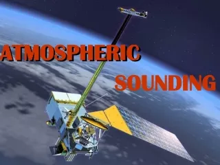
3. ATMOSPHERIC SOUNDING

4. FREQUENCY SELECTION • By measuring radiation at different frequencies or Channels with a satellite instrument a range of geophysical variables can be inferred. • In general the channels used may be considered as one of the 2 different types. • Atmospheric Sounding Channels (passive/active instruments) • Surface Sensing Channels (passive/active instruments) In practice (and often despite their name) real satellite instruments have channels which are a combination of atmospheric sounding and surface sensing.

5. ATMOSPHERIC SOUNDING CHANNELS These channels are located in parts of the infra-red and microwave spectrum for which the main contribution to the measured radiance is from the atmosphere (for which surface radiation and cloud contributions are not important)and can be written:

6. ASSUMPTIONS FOR INVERSION

8. 0.1 1.0 10.0 100.0 1000.0 668.5cm-1 676cm-1 Pressure (mb) 695cm-1 708cm-1 725cm-1 747cm-1 0.10 0.30 0.50 0.70 0.90 1.10 1.30 Weighting function (dv/d log p) Weighting function of a filter wheel vertical sounder

9. WEIGHTING FUNCTIONS OF DIFFERENT CHANNELS IN IR

10. TEMPERATURE RETRIEVAL

11. TEMPERATURE RETRIEVAL • What temperature and trace gas concentration profiles could have produced a set of observed radiances? • This is called the inverse problem or retrieval problem. • The opposite problem, called the forward problem, is to calculate outgoing radiances given temperature and trace-gas profiles.

12. RETRIEVAL METHODS • Clouds cover approximately 50% of the earth; thus about 50% of the soundings are contaminated with clouds. • Given clear-column radiances, the forward problem is easy to solve, but the retrieval problem is difficult because the solution is not unique. Even if a noise-free radiometer that measured radiances at all wavelengths could be constructed, a unique solution to the radiative transfer equation would not be guaranteed. • When a finite number of wavelengths are observed and the measurements are contaminated with noise, an infinite number of solutions are possible.

13. RETRIEVAL METHODS • The retrieval problem becomes one of finding temperature profiles that satisfy the Radiative Transfer Equation and approximate the true profiles as closely as possible. • Approaches to the retrieval problem can be classified into three general areas:- • Physical Retrieval • Statistical Retrieval • Hybrid Retrieval

14. PHYSICAL RETRIEVAL • The two most widely used methods of adjusting the temperature profile are those of Chahine (1970) and Smith (1970). • Chahine retrieves temperatures for as many levels as there are channels in the radiometer. Suppose the radiometer has J channels; then the scheme retrieves the temperature at the J levels located at the peak of the weighting functions. In this scheme there is a one-to-one correspondence between channel j of the radiometer and level J, where the weighting function of channel J peaks.

15. L - 1 <  stop the iteration L PHYSICAL RETRIEVAL METHODS In physical retrieval schemes the ease of the forward problem is exploited in an iterative process as follows:- • Step1 : A first guess temperature profile is chosen. • Step2 : The weighting functions are calculated. • Step3: The forward problem is solved to yield estimates of the radiance in each channel of the radiometer. • Step 4: If the computed radiances are the observed radiances within the noise level of the radiometer, the current profile is accepted as the solution. • Step 5: If convergence has not been achieved, the current profile is adjusted. • Step3 to 5 ( or 2 to 5) are repeated until a solution is found. • If

16. PHYSICAL RETRIEVAL METHODS • Let be Tj(n) be the nth estimate of the temperature at the Jth level and Bj(Tj(n)) be the resultant Planck radiance at level j at the wavelength of channel j. • Let Lj(n) be the nth estimate of the radiance in channel calculated using the Tj(n) and let Lj be the observed radiance in channel j. Chahine iterates the temperature by iterating the Planck radiance:

17. PHYSICAL RETRIEVAL METHODS • The iterated temperature at level j is found using the inverse Planck function. This scheme works because if, for example, the calculated radiance in channel is greater than the observed radiance, it is reasonable to adjust downward the Blanck radiance (and thus the temperature) at the level where the weighting function for channel j peaks. Since the peak of the weighting function is the highest contributor to the radiance, using the ratio of the observed to the calculated radiance to adjust the Planck radiance is also reasonable.

18. PHYSICAL RETRIEVAL METHODS • Suppose the temperature is to be retrieved at K levels. Let Tk(n) be the nth estimate of the temperature at level k, and Bj (Tk(n) ) the resulting Planck radiance at the wavelength of channel j. As above, let Lj(n) and Lj be, respectively, the nth estimate of, and the observed value of, the radiance in channel j. At each level, Smith obtains J estimates of an iterated Planck radiance: • where the J estimates of (Tk(n+1) ), obtained by the inverse Planck function, are denoted by (Tjk(n+1) ) • Not all of these J estimates are equally good because each channel sees some levels better than others.

19. PHYSICAL RETRIEVAL METHODS • Smith solves for as a weighted average of the (Tjk(n+1) ) using the weighting functions as weights. • Smith’s scheme is more flexible than that of Chahine in that it allows the user to choose the levels at which he will retrieve temperatures (consistent, of course, with the predetermined levels at which the transmittances are calculated). • However, from J channels of information, one can calculate independent temperatures at J levels at most. If K is greater than J (as is usually the case) the extra levels are not independent.

20. STATISTICAL RETRIEVAL METHODS • In statistical retrieval, the radiative transfer equation is not directly used. These methods assume that the radiometer has been designed so that its channels (weighting function) will vertically sample the atmosphere. • A set of radiosonde soundings that are nearly coincident in time & space with the satellite soundings is compiled. • This set, called the training data set, is used to calculate a statistical relationship between observed radiances and atmospheric temperatures.

21. HYBRID RETRIEVAL METHODS • Hybrid retrieval methods are in between physical and statistical retrieval methods. • They appear much like purely statistical methods, but they do not require large training data set. • They use weighting functions like physical retrievals, but they do not directly involve integration of the radiative transfer equation. • Hybrid methods are better known as inverse matrix methods.

22. RETRIEVAL OF MOISTURE PROFILES • To retrieve moisture profiles, the temperature profile is assumed, and thus B(T), is known. Smith (1970) starts with a first-guess mixing ratio profile q( p) and proceeds in a manner which is formally the same as that for temperature retrievals. The iteration formula is • is a sensitivity factor which estimates the mixing ratio change necessary to correct for a given radiance imbalance.

23. RETRIEVAL OF MOISTURE PROFILES Where U(n)(p) is the nth estimate of integrated watervapour above Pressure level p

24. NOAA/ATOVS • The Advanced TIROS Operational Vertical Sounder (ATOVS) system consists of three separate instruments, the data from with can be combined for computation of atmospheric parameters. The three instruments are: • The High Resolution Infrared Radiation Sounder (HIRS) • The Microwave Sounding Unit (AMSU) • The Stratospheric Sounding Unit (SSU) • The ATOVS can give following parameters: • 1. Temperature profiles from surface to 40Km • 2. WV content at three levels:1000-700, 700-500, 500-300 mb • 3. Outgoing Longwave Radiation (OLR) • 3. Total ozone content.

25. TEMPERATURE PROFILE

26. DEW POINT TEMPERATURE PROFILE

27. Fig.3 :Comparison of derived Temperature ( C) at 850 and 500 Mb with ATOVS and NCEP data 19 January 2001

29. ACTIVE SOUNDING USING MICROWAVES • CloudSAT • The first vertical cloud profiling from space • Cloud Profiling Radar (CPR) Carries 94 GHz nadir looking radar • CPR `slice’ through the cloud • Designed to produce three dimensional images of cloud structures • Provides information on • Cloud base and top height • Cloud water content • Cloud ice content • Cloud particle size

30. GPS FOR ATMOSPHERIC STUDIES • GPS constellation consists of 29 satellites at 26,500 km radius ~12h period orbiting in six different planes inclined at ~550 • Each GPS Satellite broadcasts two signals at L-band • f1 = 1,575.42 MHz • and • f2 = 1,227.60 MHz

31. POTENTIAL STRENGTHS OF GPS RADIO OCCULTATION TECHNIQUE • Can provide global and roughly evenly distributed coverage • Not significantly affected by clouds,precipitation or aerosols • High vertical resolution (0.1 to 0.5 km in troposphere and ~ 1.0 km in stratosphere) • No first – guess fields are required • Self-calibrating and have no instrument drift • Global Thermometer

32. VALIDATION - EXAMPLE Gadanki (13.5°N, 79.2°E): Two examples of comparison between CHAMP RO and radiosonde/lidar observations Ratnam et al., 2004, J. Atmos. Sci.