Download
1 / 83
840 likes | 1.02k Vues
Computer Science CPSC 502 Lecture 11 Probability and Time (Ch. 6.5). Where are we?. Representation. Reasoning Technique. Stochastic. Deterministic. Environment. Problem Type. Arc Consistency. Constraint Satisfaction. Vars + Constraints. Search. Static. Belief Nets.

E N D
Computer Science CPSC 502 Lecture 11 Probability and Time (Ch. 6.5)
Where are we? Representation Reasoning Technique Stochastic Deterministic • Environment Problem Type Arc Consistency Constraint Satisfaction Vars + Constraints Search Static Belief Nets Belief Nets Variable Elimination Logics Variable Elimination Query Search Approximate Inference Temporal Inference Decision Nets Sequential Variable Elimination Decision Nets STRIPS Planning Variable Elimination Belief Nets extended to cover temporal processes Search Markov Processes Markov Processes Markov Processes Value Iteration Value Iteration
Overview • Modelling Evolving Worlds with DBNs • Markov Chains • Hidden Markov Models • Inference in Temporal Models
Modeling Evolving Worlds • So far we have looked at techniques for probabilistic reasoning in a static world • E.g., keep collecting evidence to diagnose the cause of a fault in a system. • The true cause does not change as one gathers new evidence, what changes is the …………… over the possible causes.
Dynamic Bayesian Networks (DBN) • DBN are an extension of Bayesian networks devised for reasoning under uncertainty in dynamic environments • Basic approach • World’s dynamics captured via series of snapshots, or time slices, each representing the state of the world at a specific point in time • Each time slice contains a set of random variables, representing the state of the world at time t: state variables Xt • E.g., student’s knowledge and morale during a tutoring session • This assumes discrete time; step size depends on problem • Notation: Xa:b = Xa, Xa+1,…, Xb-1 , Xb Knows-Sub1 Knows-Sub3 Knows-Sub2 Knows-Add1 Knows-Add3 Knows-Add2 Morale1 Morale3 Morale2
Stationary Processes • How do we build a Bnet from these times slices and their variables? • Could use the procedure we defined for building static Bnets • order variables (temporally), • insert them in the networks one at time, • find suitable parents by checking conditional dependencies given predecessors • First Problem – we could have a very long sequence of time slices: how to specify CPTs for all of them? • Assumption of stationary process: the mechanism that regulates how state variables change overtime is stationary, that is it can be described by a single transition modelP(Xt|Xt-1) • Note that Xtis a vector representing a set of state variables
Markov Assumption • Second Problem: there could be an infinite number of parents for each node, coming from all previous time-slices • Markov assumption: current state Xt depends on bounded subset of previous states X0:t-1 • Processes satisfying this assumption are called Markov Processes or Markov Chains
Simplest Possible DBN • One random variable for each time slice: let’s assume St represents the state at time twith domain {s1 …sn} • Each random variable depends only on the previous one, thus P(St|St-1, ….S0) = • Intuitively St conveys all of the information about the history that can affect the future states. • “The future is independent of the past given the present.”
Simplest Possible DBN (cont’) • How many CPTs do we need to specify? • Stationary process assumption: the mechanism that regulates how state variables change overtime is stationary, that is it can be described by a single transition model • P(St|St-1)
Stationary Markov Chain (SMC) • A stationary Markov Chain : for all t >0 • P (St+1| S0,…,St) = P (St+1|St) • P (St +1|St) is the same for every t Markov Assumption (first order) Stationary Process • We only need to specify P (S0) and P (St +1 |St) • Simple model, easy to specify • Often the natural model • The network can extend indefinitely • Variations of SMC are at the core of most Natural Language Processing (NLP) applications!
Stationary Markov-Chain: Example Domain of variable Si is {t , q, p, a, h, e} We only need to specify… t .6 q .4 P (S0) p 0 Probability of initial state a 0 h 0 0 e Stochastic Transition Matrix t q p a h e P (St+1|St) 0 .3 0 .3 .4 0 t P (St+1| St =q) .4 0 .6 0 0 0 q 0 0 1 0 0 0 p P (St+1| St =a) 0 0 .4 .6 0 0 a 0 0 0 0 0 1 h 1 0 0 0 0 0 e
Markov-Chain: Inference P (S0,…,St) = P (S0) P (S1|S0) P (S2|S1) …………. Probability of a sequence of states S0 … ST Example: P (t,q,p) = P (St+1|St) P (S0) t .6 q .4 p 0 a 0 t q p a h e h 0 0 .3 0 .3 .4 0 t 0 e .4 0 .6 0 0 0 q 0 0 1 0 0 0 p 0 0 .4 .6 0 0 a 0 0 0 0 0 1 h 1 0 0 0 0 0 e
Key problems in NLP “I made her duck” • Assign a probability to a sentence • Part-of-speech tagging • Word-sense disambiguation, • Probabilistic Parsing • Predict the next word • Speech recognition • Hand-writing recognition • Augmentative communication for the disabled w1 w2 w3 w4 Summarization, Machine Translation…..... Impossible to estimate
Impossible to estimate! • Assuming 105 words in Dictionary and average sentence contains 10 words, how may possible worlds (entries in the JPD), would I need to specify • Google language repository (22 Sept. 2006) contained “only”: 95,119,665,584 sentences ~ 10 11 • Not enough to learn the probabilities from frequencies in this dataset (or corpus) Most sentences will not appear or appear only once
What can we do? • Make a strong simplifying assumption! • Sentences are generated by a Markov Chain P(The big red dog barks)= P(The|<S>) * These probabilities can be assessed in practice!
How can we minimally extend Markov Chains? • A useful situation to model is the one in which: • the reasoning system does not have access to the states • but can make observations that give some information about the current state
Hidden Markov Model • A Hidden Markov Model (HMM) starts with a Markov chain, and adds a noisy observation about the state at each time step: • |domain(S)| = k • |domain(O)| = h • P (S0) specifies initial conditions • P (St+1|St) specifies the dynamics • P (Ot|St) specifies the sensor model k probabilities k × k matrix of probabilities k × h matrix of probabilities • Markov Assumption on Evidence) • P(Ot|S0:t , O0:t-1) = P(Ot|St)
Simple Example (We’ll use this as a running example) • Guard stuck in a high-security bunker • Would like to know if it is raining outside • Can only tell by looking at whether his boss comes into the bunker with an umbrella every day Transition model State variables Observation model Observable variables
Discussion • Note that the first-order Markov assumption implies that the state variables contain all the information necessary to characterize the probability distribution over the next time slice • Sometime this assumption is only an approximation of reality • Whether it rains or not today may depend on the weather on more days than just the previous one • Possible fixes • Increase the order of the Markov Chain (e.g., add Raint-2 as a parent of Raint) • Add state variables that can compensate for the missing temporal information Such as?
Rain Network • We could add Month to each time slice to include season statistics Montht Montht+1 Montht-1 Raint+1 Raint-1 Raint Umbrellat+1 Umbrellat-1 Umbrellat
Pressuret+1 Pressuret Pressuret-1 Humidityt+1 Humidityt Humidityt-1 Temperaturet+1 Temperaturet Temperaturet-1 Raint-1 Raint Raint+1 Umbrellat-1 Umbrellat Umbrellat+1 Rain Network • Or we could add Temperature, Humidity and Pressure toinclude meteorological knowledge in the network
Rain Network • However, adding more state variables may require modelling their temporal dynamics in the network • Trick to get away with it • Add sensors that can tell me the value of each new variable at each specific point in time • The more reliable a sensor, the less important to include temporal dynamics to get accurate estimates of the corresponding variable Humidityt Humidityt-1 Pressuret-1 Pressuret Temperaturet-1 Temperaturet Raint Raint-1 Thermometert Thermometert-1 Barometert-1 Barometert Umbrellat Umbrellat-1
Overview • Modelling Evolving Worlds with DBNs • Marcov Chains • Hidden Markov Models • Inference in Temporal Models
Inference Tasks in Temporal Models • Filtering (or monitoring): P(Xt|e0:t) • Compute the posterior distribution over the current state given all evidence to date • In the rain example, this would mean computing the probability that it rains today given all the observations on umbrella made so far • Important if a rational agent needs to make a decision in the current situation • Prediction: P(Xt+k| e0:t) • Compute the posterior distribution over a future state given all evidence to date • In the rain example, this would mean computing the probability that it rains in two days given all the observations on umbrella made so far • Useful for an agent to evaluate possible courses of actions
Inference Tasks in Temporal Models • Smoothing: P(Xt-k| e0:t) • Compute the posterior distribution over a past state given all evidence to date • In the rain example, this would mean computing the probability that it rained five days ago given all the observations on umbrella made so far • Useful to better estimate what happened by incorporating additional evidence to the evidence available at that time • Most Likely Explanation: argmaxX0:tP(X0:t| e0:t) • Given a sequence of observations, find the sequence of states that is most likely to have generated them • Useful in many applications, e.g., speech recognition: find the most likely sequence of words given a sequence of sounds
Filtering • Idea: recursive approach • Compute filtering up to time t-1, and then include the evidence for time t (recursive estimation) TRUE 0.5 FALSE 0.5 Rain2 Rain0 Rain1 Umbrella2 Umbrella1
Filtering • Idea: recursive approach • Compute filtering up to time t-1, and then include the evidence for time t (recursive estimation) • P(St | o0:t) = P(St | o0:t-1,ot) dividing up the evidence = α P(ot| St, o0:t-1) P(St | o0:t-1) WHY? = αP(ot| St) P(St| o0:t-1) WHY? Prediction of current state given evidence up to t-1 Inclusion of new evidence: this is available from.. • So we only need to computeP(St| o0:t-1)
why? Filtering Product Rule P(A,B) = P(A|B)P(B) • Compute P(St| o0:t-1) • P(St| o0:t-1) = ∑St-1P(St, St-1 |o0:t-1) = ∑St-1P(St| St-1 , o0:t-1) P( St-1 | o0:t-1) = • = ∑St-1P(St| St-1 ) P( St-1 | o0:t-1) because of.. Filtering at time t-1 Transition model! • Putting it all together, we have the desired recursive formulation • P(St | o0:t) = αP(ot| St) ∑St-1P(St| St-1 ) P( St-1 | o0:t-1) Filtering at time t-1 Inclusion of new evidence (sensor model) Propagation to time t • P( St-1 | o0:t-1) can be seen as a message f0:t-1 that is propagated forward along the sequence, modified by each transition and updated by each observation
Filtering • Thus, the recursive definition of filtering at time t in terms of filtering at time t-1 can be expressed as a FORWARD procedure • f0:t =α FORWARD (f0:t-1, ot) • which implements the update described in P(St | o0:t) = αP(ot| St) ∑St-1P(St| St-1 ) P( St-1 | o0:t-1) Filtering at time t-1 Inclusion of new evidence (sensor model) Propagation to time t
Analysis of Filtering • Because of the recursive definition in terms for the forward message, when all variables are discrete the time for each update is constant (i.e. independent of t) • The constant depends of course on the size of the state space and the type of temporal model
Rain Example • Suppose our security guard came with a prior belief of 0.5 that it rained on day 0, just before the observation sequence started. • Without loss of generality, this can be modeled with a fictitious state R0 with no associated observation and P(R0) = <0.5, 0.5> • P(R1| o0:t-1) = P(R1) = ∑r0P(R1 | r0 ) P(r0 ) • = <0.7, 0.3> * 0.5 + <0.3,0.7> * 0.5 = <0.5,0.5> • Day 1: umbella appears (u1). Thus 0.5 0.5 TRUE 0.5 FALSE 0.5 Rain2 Rain0 Rain1 Umbrella2 Umbrella1
Rain Example • Updating P(R1) with evidence from for t =1 (umbrella appeared) gives • P(R1| u1) = α P(u1 | R1) P(R1) = • α<0.9, 0.2><0.5,0.5> = α<0.45, 0.1> ~ <0.818, 0.182> • Day 2: umbella appears (u2). Thus • P(R2 | o0:t-1) = P(R2 | u1 ) = ∑r1P(R2 | r1 ) P(r1 | u1) = • = <0.7, 0.3> * 0.818 + <0.3,0.7> * 0.182 ~ <0.627,0.373> Vector dot product 0.627 0.373 0.5 0.5 TRUE 0.5 FALSE 0.5 0.818 0.182 Rain2 Rain0 Rain1 Umbrella2 Umbrella1
Rain Example • Updating this with evidence from for t =2 (umbrella appeared) gives • P(R2| u1 , u2) = αP(u2| R2) P(R2| u1) = • α<0.9, 0.2><0.627,0.373> = α<0.564, 0.075> ~ <0.883, 0.117> • Intuitively, the probability of rain increases, because the umbrella appears twice in a row 0.627 0.373 0.5 0.5 TRUE 0.5 FALSE 0.5 0.883 0.117 0.818 0.182 Rain2 Rain0 Rain1 Umbrella2 Umbrella1
Prediction: P(St+k+1| o0:t ) • Can be seen as filtering without addition of new evidence • In fact, filtering already contains a one-step prediction • P(St | o0:t) = αP(ot| St) ∑st-1P(St| st-1 ) P( st-1 | e0:t-1 ) Filtering at time t-1 Inclusion of new evidence (sensor model) Propagation to time t • We just need to show how to recursively predict the state at time t+k +1 from a prediction for state t + k • P(St+k+1| o0:t) = ∑st+kP(St+k+1, st+k|o0:t) = ∑st+kP(St+k+1| st+k, o0:t) P( st+k| o0:t) = • = ∑st+kP(St+k+1| st+k) P( st+k| o0:t) • Let‘s continue with the rain example and compute the probability of Rain on day four after having seen the umbrella in day one and two: P(R4| u1 , u2) Prediction for state t+ k Transition model
Rain Example • Prediction from day 2 to day 3 • P(S3| o1:2) = ∑s2P(S3| s2 ) P( s2 | o1:2) = ∑r2P(R3 | r2 ) P( r2 | u1 u2 ) = • = <0.7,0.3>*0.883 + <0.3,0.7>*0.117 = <0.618,0.265> + <0.035, 0.082> • = <0.653, 0.347> • Prediction from day 3 to day 4 • P(S4| o1:2) = ∑s3P(S4| s3 ) P( s3 | o1:2) = ∑r3P(R4 | r3 ) P( r3 | u1 u2 ) = • = <0.7,0.3>*0.653 + <0.3,0.7>*0.347= <0.457,0.196> + <0.104, 0.243> • = <0.561, 0.439> 0.627 0.373 0.5 0.5 0.561 0.439 0.653 0.347 0.5 0.5 0.883 0.117 0.818 0.182 Rain3 Rain3 Rain0 Rain1 Rain2 Umbrella3 Umbrella1 Umbrella2 Umbrella3
Rain Example • Intuitively, the probability that it will rain decreases for each successive day, as the influence of the observations from the first two days decays • What happens if I try to predict further and further into the future? • It can be shown that the predicted distribution converges to the stationary distribution of the Markov process defined by the transition model (<0.5,0.5> for the rain example) • When the convergence happens, I have basically lost all the information provided by the existing observations, and I can’t generate any meaningful prediction on states from this point on • The time necessary to reach this point is called mixing time. • The more uncertainty there is in the transition model, the shorter the mixing time will be • Basically, the more uncertainty there is in what happens at t+1 given that I know what happens in t, the faster the information that I gain from evidence on the state at t dissipates with time
Another Example: Localization for “Pushed around” Robot • Localization (where am I?) is a fundamental problem in robotics • Suppose a robot is in a circular corridor with 16 locations • There are four doors at positions: 2, 4, 7, 11 • The Robot initially doesn’t know where it is • The Robot is pushed around. After a push it can stay in the same location, move left or right. • The Robot has a noisy sensor telling whether it is in front of a door
This scenario can be represented as… • Example Stochastic Dynamics: when pushed, it stays in the same location p=0.2, moves left or right with equal probability P(Loct + 1 | Loct) 0 1 2 .. 15 16 0.4 0.4 0.4 0.2 . . 0.4 0 . 0.2 . 1 2 P(Loc0) 3 .. 1/16 for each location in the corridor 0.2 16
This scenario can be represented as… • Example of Noisy sensor telling whether it is in front of a door. • If it is in front of a door P(O t = T) = .8 • If not in front of a door P(O t = T) = .1 P(O t | Loct)
Useful inference in this problem • Localization: Robot starts at an unknown location and it is pushed around t times. It wants to determine where it is P(Loct| o0, o1,…,o t) • This is an instance of Filtering: • compute the posterior distribution over the current state given all evidence to date • P(St | o0:t)
More complex Example: Robot Localization • Suppose a robot wants to determine its location based on its actions and its sensor readings • Three actions: goRight, goLeft, Stay • This can be represented by an augmented HMM
Robot Localization Sensor and Dynamics Model • Sample Sensor Model (assume same as for pushed around) • Sample Stochastic Dynamics: P(Loct + 1 | Actiont, Loc t) P(Loct + 1 = L | Action t = goRight , Loc t = L) = 0.1 P(Loct + 1 = L+1 | Action t = goRight , Loc t = L) = 0.8 P(Loct + 1 = L + 2 | Action t = goRight , Loc t = L) = 0.074 P(Loct + 1 = L’ | Action t = goRight , Loc t = L) = 0.002 for all other locations L’ • All location arithmetic is modulo 16 • The action goLeft works the same but to the left • The action Stay is deterministic
Dynamics Model More Details • Sample Stochastic Dynamics: P(Loct + 1 | Action, Loc t) P(Loct + 1 = L | Action t = goRight , Loc t = L) = 0.1 P(Loct + 1 = L+1 | Action t = goRight , Loc t = L) = 0.8 P(Loct + 1 = L + 2 | Action t = goRight , Loc t = L) = 0.074 P(Loct + 1 = L’ | Action t = goRight , Loc t = L) = 0.002 for all other locations L’ 0 0 1 1 2 2 .. .. 15 15 16 16 . . . . 0 0 . . . . 1 1 2 2 3 3 .. .. 16 16
Example Inference What is the probability distribution for the robot location at time 2, given the following sequence of observations and actions
Robot Localization additional sensor • Additional Light Sensor: there is light coming through an opening at location 10. The light sensor detects if there is light or not at a given location. • What do we need to specify?
Robot Localization additional sensor • Additional Light Sensor: there is light coming through an opening at location 10 P (Lt | Loct) P (Lt =t) P (Lt =f) • Info from the two sensors is combined :“Sensor Fusion” • Do we need to do anything special to make this sensor fusion happen?
The Robot starts at an unknown location and must determine where it is • The model appears to be too ambiguous • Sensors are too noisy • Dynamics are too stochastic to infer anything But inference actually works pretty well. check: http://artint.info/demos/localization/localization.html It uses a generalized form of filtering (not just a sequence of observations, but a sequence of observation pairs (from the two sensors) + the actions
HMMs have many other applications…. • Natural Language Processing: e.g., Speech Recognition • States: phoneme \ word • Observations: acoustic signal \ phoneme • Bioinformatics: Gene Finding • States: coding / non-coding region • Observations: DNA Sequences For these problems the critical inference is: find the most likely sequence of states given a sequence of observations
Most Likely Sequence • Suppose that in the rain example we have the following umbrella observation sequence • [true, true, false, true, true] • Is it the perfect reflection on the rain situation? • [rain, rain, no-rain, rain, rain] • Or perhaps it did rain on the third day but the boss forgot to bring the umbrella? • If it did not rain on day 3, perhaps it also did not rain on day 4, but the boss brought the umbrella just in case • 25 possible sequences of states
Most Likely Sequence (Explanation) • Most Likely Sequence: argmaxx0:tP(X0:t| e0:t) • General idea: search in a graph whose nodes are the possible states at each time step