Download

1 / 68
680 likes | 842 Vues
Computer Science CPSC 502 Lecture 12 Decisions Under Uncertainty (Ch. 9, up to 9.3). Representational Dimensions. Representation. Environment. Reasoning Technique. Stochastic. Deterministic. Problem Type. Arc Consistency.

E N D
Computer Science CPSC 502 Lecture 12 Decisions Under Uncertainty (Ch. 9, up to 9.3)
Representational Dimensions Representation • Environment Reasoning Technique Stochastic Deterministic Problem Type Arc Consistency This concludes the module on answering queries in stochastic environments Constraint Satisfaction Vars + Constraints Search Static Belief Nets Logics Variable Elimination Query Search Approximate Temporal Inference Sequential Decision Nets STRIPS Variable Elimination Search Planning Markov Processes Value Iteration
Representational Dimensions Representation • Environment Reasoning Technique Stochastic Deterministic Problem Type Arc Consistency Constraint Satisfaction Now we will look at acting in stochastic environments Vars + Constraints Search Static Belief Nets Logics Variable Elimination Query Search Approximate Temporal Inference Sequential Decision Nets STRIPS Variable Elimination Search Planning Markov Processes Value Iteration
Lecture Overview • Single-Stage Decision Problems • Utilities and optimal secisions • Single-Stage decision networks • Variable elimination (VE) for computing the optimal decision • Sequential Decision Problems • General decision networks • Policies • Finding optimal policies with VE
Decisions Under Uncertainty: Intro • Earlier in the course, we focused on decision making in deterministic domains • Search/CSPs: single-stage decisions • Planning: sequential decisions • Now we face stochastic domains • so far we've considered how to represent and update beliefs • what if an agent has to make decisions (act) under uncertainty? • Making decisions under uncertainty is important • We represent the world probabilistically so we can use our beliefs as the basis for making decisions
Decisions Under Uncertainty: Intro • An agent's decision will depend on • What actions are available • What beliefs the agent has • Which goals the agent has • Differences between deterministic and stochastic setting • Obvious difference in representation: need to represent our uncertain beliefs • Actions will be pretty straightforward: represented as decision variables • Goals will be interesting: we'll move from all-or-nothing goals to a richer notion: • rating how happy the agent is in different situations. • Putting these together, we'll extend Bayesian Networks to make a new representation called Decision Networks
Delivery Robot Example • Robot needs to reach a certain room • Robot can go • the short way - faster but with more obstacles, thus more prone to accidents that can damage the robot • the long way - slower but less prone to accident • Which way to go? Is it more important for the robot to arrive fast, or to minimize the risk of damage? • The Robot can choose to wear pads to protect itself in case of accident, or not to wear them. Pads slow it down • Again, there is a tradeoff between reducing risk of damage and arriving fast • Possible outcomes • No pad, no accident • Pad, no accident • Pad, Accident • No pad, accident
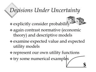
Next • We’ll see how to represent and reason about situations of this nature using Decision Trees, as well as • Probability to measure the uncertainty in action outcome • Utility to measure agent’s preferences over the various outcomes • Combined in a measure of expected utility that can be used to identify the action with the best expected outcome • Best that an intelligent agent can do when it needs to act in a stochastic environment
Decision Tree for the Delivery Robot Example • Decision variable 1: the robot can choose to wear pads • Yes: protection against accidents, but extra weight • No: fast, but no protection • Decision variable 2: the robot can choose the way • Short way: quick, but higher chance of accident • Long way: safe, but slow • Random variable: is there an accident? Agent decides Chance decides
Delivery Robot Example • Decision variable 1: the robot can choose to wear pads • Yes: protection against accidents, but extra weight • No: fast, but no protection • Decision variable 2: the robot can choose the way • Short way: quick, but higher chance of accident • Long way: safe, but slow • Random variable: is there an accident? Agent decides Chance decides
Possible worlds and decision variables • A possible world specifies a value for each random variable and each decision variable • For each assignment of values to all decision variables • the probabilities of the worlds satisfying that assignment sum to 1. 0.2 0.8
Possible worlds and decision variables • A possible world specifies a value for each random variable and each decision variable • For each assignment of values to all decision variables • the probabilities of the worlds satisfying that assignment sum to 1. 0.2 0.8 0.01 0.99
Possible worlds and decision variables • A possible world specifies a value for each random variable and each decision variable • For each assignment of values to all decision variables • the probabilities of the worlds satisfying that assignment sum to 1. 0.2 0.8 0.01 0.99 0.2 0.8
Possible worlds and decision variables • A possible world specifies a value for each random variable and each decision variable • For each assignment of values to all decision variables • the probabilities of the worlds satisfying that assignment sum to 1. 0.2 0.8 0.01 0.99 0.2 0.8 0.01 0.99
Utility • Utility: a measure of desirability of possible worlds to an agent • Let U be a real-valued function such that U(w) represents an agent's degree of preference for world w • Expressed by a number in [0,100] • Simple goals can still be specified • Worlds that satisfy the goal have utility 100 • Other worlds have utility 0 • Utilities can be more complicated • For example, in the robot delivery domains, they could involve • Reached the target room? • Time taken • Amount of damage • Energy left
Utility for the Robot Example • Which would be a reasonable utility function for our robot? • Which are the best and worst scenarios? probability Utility 0.2 0.8 0.01 0.99 0.2 0.8 0.01 0.99
Utility / Preferences • Utility: a measure of desirability of possible worlds to an agent • Let U be a real-valued function such that U (w) represents an agent's degree of preference for world w. Would this be a reasonable utility function for our Robot?
Utility: Simple Goals • Can simple (boolean) goals still be specified?
Utility for the Robot Example • Now, how do we combine utility and probability to decide what to do? probability Utility 0.2 35 35 95 0.8 35 30 0.01 75 0.99 0.2 35 3 100 0.8 35 0 0.01 80 0.99
Optimal decisions: combining Utility and Probability • Each set of decisions defines a probability distribution over possible outcomes • Each outcome has a utility • For each set of decisions, we need to know their expected utility • the value for the agent of achieving a certain probability distribution over outcomes (possible worlds) 0.2 35 95 0.8 value of this scenario? • The expected utility of a set of decisions is obtained by • weighting the utility of the relevant possible worlds by their probability. • We want to find the decision with maximum expected utility
Expected utility of a decision • The expected utility of decision D = di is • What is the expected utility of Wearpads=yes, Way=short ? E(U | D = di) =w╞ (D = di)P(w) U(w) probability Utility E[U|D] 0.2 35 35 95 0.8 30 35 0.01 75 0.99 0.2 35 3 100 0.8 35 0 0.01 80 0.99
Expected utility of a decision • The expected utility of decision D = di is • What is the expected utility of Wearpads=yes, Way=short ? • 0.2 * 35 + 0.8 * 95 = 83 E(U | D = di) =w╞ (D = di)P(w) U(w) probability Utility E[U|D] 0.2 35 35 83 95 0.8 35 30 0.01 74.55 75 0.99 0.2 35 3 80.6 100 0.8 35 0 0.01 79.2 80 0.99
Lecture Overview • Single-Stage Decision Problems • Utilities and optimal secisions • Single-Stage decision networks • Variable elimination (VE) for computing the optimal decision • Sequential Decision Problems • General decision networks • Policies • Finding optimal policies with VE
Single Action vs. Sequence of Actions • Single Action (aka One-Off Decisions) • One or more primitive decisions that can be treated as a single macro decision to be made before acting • E.g., “WearPads” and “WhichWay” can be combined into macro decision (WearPads, WhichWay) with domain {yes,no} × {long, short} • Sequence of Actions (Sequential Decisions) • Repeat: • make observations • decide on an action • carry out the action • Agent has to take actions not knowing what the future brings • This is fundamentally different from everything we’ve seen so far • Planning was sequential, but we still could still think first and then act
Optimal single-stage decision • Given a single (macro) decision variable D • the agent can choose D=difor any value di dom(D)
What is the optimal decision in the example? Conditional probability Which is the optimal decision here? Utility E[U|D] 0.2 35 35 83 95 0.8 35 30 0.01 74.55 75 0.99 0.2 35 3 80.6 100 0.8 35 0 0.01 79.2 80 0.99
Optimal decision in robot delivery example Best decision: (wear pads, short way) Conditional probability Utility E[U|D] 0.2 35 35 83 95 0.8 30 35 0.01 74.55 75 0.99 0.2 35 3 80.6 100 0.8 35 0 0.01 79.2 80 0.99
Single-Stage decision networks • Extend belief networks with: • Decision nodes, that the agent chooses the value for • Parents: only other decision nodes allowed • Domain is the set of possible actions • Drawn as a rectangle • Exactly one utility node • Parents: all random & decision variables on which the utility depends • Does not have a domain • Drawn as a diamond • Explicitly shows dependencies • E.g., which variables affect the probability of an accident?
Types of nodes in decision networks • A random variable is drawn as an ellipse. • Arcs into the node represent probabilistic dependence • As in Bayesian networks: a random variable is conditionally independent of its non-descendants given its parents • A decision variable is drawn as an rectangle. • Arcs into the node represent information available when the decision is made • A utility node is drawn as a diamond. • Arcs into the node represent variables that the utility depends on. • Specifies a utility for each instantiation of its parents
Example Decision Network Decision nodes do not have an associated table. The utility node does not have a domain.
Computing the optimal decision: we can use VE • Denote • the random variables as X1, …, Xn • the decision variables as D • the parents of node N as pa(N) • To find the optimal decision we can use VE: • Create a factor for each conditional probability and for the utility • Sum out all random variables, one at a time • This creates a factor on D that gives the expected utility for each di • Choose the di with the maximum value in the factor
Computing the optimal decision: we can use VE • Denote • the random variables as X1, …, Xn • the decision variables as D • the parents of node N as pa(N) • To find the optimal decision we can use VE: • Create a factor for each conditional probability and for the utility • Sum out all random variables, one at a time • This creates a factor on D that gives the expected utility for each di • Choose the di with the maximum value in the factor Includes decision vars
VE Example: Step 1, create initial factors f1(A,W) Abbreviations: W = Which WayP = Wear PadsA = Accident f2(A,W,P)
VE example: step 2, sum out A Step 2a: compute product f(A,W,P) = f1(A,W) × f2(A,W,P) f(A=a,P=p,W=w) = f1(A=a,W=w) × f2(A=a,W=w,P=p)
VE example: step 2, sum out A Step 2a: compute product f(A,W,P) = f1(A,W) × f2(A,W,P) f(A=a,P=p,W=w) = f1(A=a,W=w) × f2(A=a,W=w,P=p)
VE example: step 2, sum out A The final factor encodes the expected utility of each decision Step 2b: sum A out of the product f(A,W,P):
VE example: step 2, sum out A The final factor encodes the expected utility of each decision Step 2b: sum A out of the product f(A,W,P):
Expected utility of a decision • The expected utility of decision D = di is • What is the expected utility of Wearpads=yes, Way=short ? • 0.2 * 35 + 0.8 * 95 = 83 E(U | D = di) =w╞ (D = di)P(w) U(w) probability Utility E[U|D] 0.2 35 35 83 95 0.8 35 30 0.01 74.55 75 0.99 0.2 35 3 80.6 100 0.8 35 0 0.01 79.2 80 0.99
VE example: step 2, sum out A Step 2b: sum A out of the product f(A,W,P): The final factor encodes the expected utility of each decision
VE example: step 3, choose decision with max E(U) The final factor encodes the expected utility of each decision • Thus, taking the short way but wearing pads is the best choice, with an expected utility of 83 Step 2b: sum A out of the product f(A,W,P):
Variable Elimination for Single-Stage Decision Networks: Summary • Create a factor for each conditional probability and for the utility • Sum out all random variables, one at a time • This creates a factor on D that gives the expected utility for each di • Choose the di with the maximum value in the factor
Lecture Overview • Single-Stage Decision Problems • Utilities and optimal secisions • Single-Stage decision networks • Variable elimination (VE) for computing the optimal decision • Sequential Decision Problems • General decision networks • Policies • Finding optimal policies with VE
Sequential Decision Problems • An intelligent agent doesn't make a multi-step decision and carry it out blindly • It would take new observations it makes into account • A more typical scenario: • The agent observes, acts, observes, acts, … • Subsequent actions can depend on what is observed • What is observed often depends on previous actions • Often the sole reason for carrying out an action is to provide information for future actions • For example: diagnostic tests, spying • General Decision networks: • Just like single-stage decision networks, with one exception:the parents of decision nodes can include random variables
Sequential decisions : Simplest possible • Only one decision! (but different from one-off decisions) • Early in the morning. Shall I take my umbrella today? (I’ll have to go for a long walk at noon) • Relevant Random Variables?
Sequential Decision Problems: Example • In our Fire Alarm domain • If there is a report you can decide to call the fire department • Before doing that, you can decide to check if you can see smoke, but this takes time and will delay calling • A decision (e.g. Call) can depends ona random variable (e.g. SeeSmoke ) • Each decision Di has an information set of variables pa(Di), whose value will be known at the time decision Di is made • pa(CheckSmoke) = {Report} • pa(Call) = {Report, CheckSmoke, See Smoke} Decision node: Agent decides Chance node: Chance decides
Sequential Decision Problems • What should an agent do? • The agent observes, acts, observes, acts, … • Subsequent actions can depend on what is observed • What is observed often depends on previous actions • The agent needs a conditional plan of what it will do given every possible set of circumstances • We will formalize this conditional plan as a policy
Policies for Sequential Decision Problems Definition (Policy)A policy is a sequence of δ1 ,…..,δn decision functions δi : dom(pa(Di )) → dom(Di) This policy means that when the agent has observed odom(pa(Di )) , it will do δi(o) There are 22=4 possible decision functions δcsfor Check Smoke: - Decision function needs to specify a value for each instantiation of parents CheckSmoke
Policies for Sequential Decision Problems Definition (Policy)A policy is a sequence of δ1 ,…..,δn decision functions δi : dom(pa(Di )) → dom(Di) This policy means that when the agent has observed odom(pa(Di )) , it will do δi(o) There are 22=4 possible decision functions δcsfor Check Smoke: - Decision function needs to specify a value for each instantiation of parents CheckSmoke
Policies for Sequential Decision Problems Definition (Policy)A policy is a sequence of δ1 ,…..,δn decision functions δi : dom(pa(Di )) → dom(Di) when the agent has observed odom(pDi) , it will do δi(o) There are possible decision functions δcsfor Call:
Policies for Sequential Decision Problems Definition (Policy)A policy is a sequence of δ1 ,…..,δn decision functions δi : dom(pa(Di )) → dom(Di) when the agent has observed odom(pDi) , it will do δi(o) There are 28=256 possible decision functions δcsfor Call: