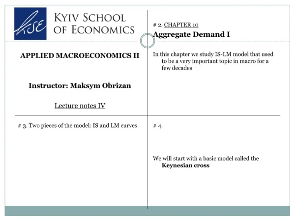
APPLIED MACROECONOMICS II Instructor: Maksym Obrizan Lecture notes IV
APPLIED MACROECONOMICS II Instructor: Maksym Obrizan Lecture notes IV. # 2. CHAPTER 10 Aggregate Demand I In this chapter we study IS-LM model that used to be a very important topic in macro for a few decades. # 3. Two pieces of the model: IS and LM curves. # 4.

APPLIED MACROECONOMICS II Instructor: Maksym Obrizan Lecture notes IV
E N D
Presentation Transcript
APPLIED MACROECONOMICS II Instructor: MaksymObrizan Lecture notes IV # 2. CHAPTER 10 Aggregate Demand I In this chapter we study IS-LM model that used to be a very important topic in macro for a few decades # 3. Two pieces of the model: IS and LM curves # 4. We will start with a basic model called the Keynesian cross
# 5. Actual and planned expenditure Actual expenditure – Planned expenditure - # 6. Why do actual and planned expenditure differ? # 7. A general form for planned expenditure # 8. A textbook example
# 9. # 10. Deriving Keynesian cross The economy is in equilibrium when actual expenditure equals planned expenditure # 11. # 12. How does the economy adjust to equilibrium?
# 13. # 14. Fiscal policy and government multiplier An increase in government purchases G leads to greater increase in income Y # 15. Why does fiscal policy have a multiplied effect on income? # 16. Computing the multiplier
# 17. Numerical example # 18. # 19. An Increase in Government Purchases in the Keynesian Cross # 20. The Interest Rate, Investment, and the IS Curve When we introduced the Keynesian cross we assumed that investment I is fixed We can write the level of planned investment as I = I(r)
# 21. Deriving the IS curve # 22. Figure for the Keynesian Cross # 23. The Investment Function # 24. The IS curve
# 25. IS curve and fiscal policy The IS curve is drawn for a given fiscal policy # 26. The Keynesian cross with increase in G # 27. An Increase in Government Purchases Shifts the IS Curve Outward Panel # 28. The IS curve after increase in G
# 29. The Money Market and the LM Curve The LM curve plots the relationship between the interest rate and the level of income that arises in the market for money balances. # 30. Supply of real money balances # 31. The supply of real money balances against the interest rate is a vertical supply curve. # 32. Demand for real money balances The interest rate is the opportunity cost of holding money
# 33. Figure 10-10 # 34. A Reduction in the Money Supply in the Theory of Liquidity Preference # 35. Figure 10-11 # 36. Income, Money Demand, and the LM Curve
# 37. The Market for Real Money Balances # 38. The LM curve # 39. Deriving the LM curve # 40.
# 41. Monetary policy and the LM curve # 42. Decrease in supply of real money balances # 43. The Market for Real Money Balances # 44. The LM Curve
# 45. The IS-LM curve The IS-LM model assumes that fiscal policy, G and T, monetary policy M, and the price level P are exogenous. # 46. Deriving the equilibrium # 47. Figure 10-14 # 48. Implications

