Efficient Dynamic Aggregation
Efficient Dynamic Aggregation. Yitzhak Birk , Idit Keidar , Liran Liss, Assaf Schuster Technion. Dynamic Aggregation. Continuous monitoring of aggregate value over changing inputs Examples: More than 10% of sensors report of seismic activity Maximum temperature in data center

Efficient Dynamic Aggregation
E N D
Presentation Transcript
Efficient Dynamic Aggregation Yitzhak Birk, Idit Keidar,Liran Liss, Assaf Schuster Technion
Dynamic Aggregation • Continuous monitoring of aggregate value over changing inputs • Examples: • More than 10% of sensors report of seismic activity • Maximum temperature in data center • Average load in computation grid
The Setting • Large graph (e.g., sensor network) • Direct communication only between neighbors • Each node has a changing input • Inputs change more frequently than topology • Consider topology as static • Aggregate function f on multiplicity of inputs • Oblivious to locations • Aggregate result computed at all nodes
Goals for Dynamic Aggregation • Fast convergence • If from some time t onward inputs do not change … • Output stabilization time from t • Quiescence time from t • Note: nodes do not know when stabilization and quiescence are achieved • If after stabilization input changes abruptly… • Efficient communication • Zero communication when there are zero changes • Small changes little communication
Standard Aggregation Solution: Spanning Tree 20 black, 12 white Global communication! black! 7 black, 1 white black! 2 black 1 black
Spanning Tree: Value Change 19 black, 13 white Global communication! 6 black, 2 white
The Bad News • Virtually every aggregation function has instances that cannot be computed without communicating with the whole graph • E.g., majority voting when close to the threshold “every vote counts” • Worst case analysis: convergence, quiescence times are (diameter)
Instance-Locality to the Rescue • Although some instances require global computation, most can stabilize (and become quiescent) locally • In small neighborhood, independent of graph size • Shown empirically [Wolff,Schuster03, Liss,Birk,Wolf,Schuster04] • Formal instance-based locality in other contexts • Local fault mending [Kutten,Peleg95, Kutten,Patt-Shamir97] • Growth-restricted graphs [Kuhn, Moscibroda, Wattenhofer05] • MST [Elkin04]
“Per-Instance” Optimality Too Strong • Instance: assignment of inputs to nodes • For a given instance I, algorithm AIdoes: • if (my input is as in I) output f(I)else send message with input to neighbor • Upon receiving message, flood it • Upon collecting info from the whole graph, output f(I) • Convergence and output stabilization in zero time on I • Can you beat that? Need to measure optimality per-class notper-instance Challenge: capture attainable locality
Veracity Radius (VR) for One-Shot Aggregation [BKLSW,PODC’06] • Roughly speaking: the min radius r0 such that"r> r0: all r-neighborhoods have same result • Example: majority Radius 1: wrong result Radius 2: correct result VR=2
Veracity Radius Captures the Locality of One-Shot Aggregation [BKLSW,PODC’06] • Class-based lower bound • Both output stabilization and quiescence • For every r, for every algorithm A, there is an instance I with VR(I) r on which A takes r time • I-LEAG (Instance-Local Efficient Aggregation on Graphs) • Quiescence and output stabilization proportional to VR • Per-class within a factor of optimal • Local: depends on VR, not graph size! • Note: nodes do not know VR or when stabilization and quiescence are achieved • Can’t expect to know you’re “done” in dynamic aggregation…
Naïve Dynamic Aggregation • Periodically, • Each node samples input, initiates I-LEAG • Each instance I of I-LEAG takes O(VR(I)) time, but sends (|V|) messages • Sends messages even when no input changes • Costly in sensor networks • To save messages, must compromise freshness of result
Contributions • New lower bound • For algorithms that send zero messages when there are zero changes • Efficient multi-shot aggregation algorithm (MultI-LEAG) • Converges to correct result before sampling the inputs again • Sampling time may be proportional to graph size • Efficient dynamic aggregation algorithm (DynI-LEAG) • Sampling time is independent of graph size • Algorithm tracks global result as close as possible
Dynamic Lower Bound • Previous sample (instance) also plays a role • Example (majority voting): • Multi-shot lower bound:max{VRprev,VR} • On quiescence and output stabilization • Assumes sending zero messages when there are zero changes I2 (0 changes) I1 (VR2) ! ? I3 (VR=0)
Dynamic Aggregation: Take II • Initially, run local one-shot algorithm A • Store distance information travels in this instance, dist • Let D = A’s worst-case convergence time • Every D time, run a new iteration (MULTI-A) • If input did not change, do nothing • If input changed, run full information protocol up to dist • If new instance’s VR isn’t reached, invoke A anew • Update dist (~VR) • (~ VRprev) (~VR) • Matches max{VRprev,VR} lower bound • within same factor as A
A is for I-LEAG • I-LEAG uses a pre-computed partition hierarchy • LPH: Local Partition Hierarchy – cluster sizes bounded both from above and from below (doubling sizes) • Spanning tree in each cluster, rooted at pivot • Computed once per topology • I-LEAG phases correspond to LPH levels • Active phase: full-information from cluster pivot • Phase result communicated to cluster and its neighbors • Phase active only if there is a conflict in the previous level • Conflicts detected without new communication
Multi-LEAG • The Veracity Level (VL) of node v is the highest LPH level in which v’s cluster has a conflict (VL<logVR+1) • A multi-LEAG iteration’s phases correspond to LPH levels: • Phase level < VL: propagate changes (if any) to pivot • active only if there are changes • Phase level VL: fall back to I-LEAG • active only if new VR is larger than previous • Cache partial aggregate results in pivot nodes • allows conflict detection between active and passive clusters
MultI-LEAG Operation Veracity Level Pivot nodes Physical nodes
MultI-LEAG Operation • Case I: No changes … no conflicts … no conflicts … no changes to report All is quiet…
Input Change no conflicts, no communication New veracity level !
Abrupt Change Flips Outcome Clusters at VL recalculate, others forward up
Abrupt Change Flips Outcome no conflicts, no communication New Veracity level
MultI-LEAG Observations • O(max{VRprev,VR}) output stabilization and quiescence • Message efficient: • Communication only in clusters with changes, only when radius < max{VRprev,VR} • Sampling time is O(Diameter) • Good for cheap periodic aggregation • Can we do closer monitoring?
Dynamic Aggregation Take III: DynI-LEAG • Sample inputs every O(1) link delays • Close monitoring, rapidly converges to correct result • Run multiple MultI-LEAG iterations concurrently • Challenges: • Pipelining phases with different (doubling) durations • Intricate interaction among concurrent instancesE.g., which phase 4 updates are used in a given phase 5 .. • Avoiding state explosion for multiple concurrent instances
Ruler Pipelining • Partial iterations, fewer in every level • Changes only communicated once Full iteration Sampling interval Phase 2 Partial iteration Phase 1 Phase 0 t • Memory usage: O(log(Diameter))
VL and Output Estimation • Problem: correct output and VL of an iteration is guaranteed only after O(Diameter) time • cannot wait that long… • Solution: choose iteration with highest VL according to most recent information • Use this VL for new iterations and its output as MultI-LEAG’s current output estimation • Eventual convergence and correctness guaranteed
DynI-LEAG Operation The influence of a conflict is proportional to its level Phase below VL Phase above VL 2 1 0 t “Previous VL” = 2
Conclusions • Local operation is possible • in dynamic systems • that solve inherently global problems • MultI-LEAG delivers periodic correct snapshots at minimal cost • DynI-LEAG responds immediately to input changes with a slightly higher message rate