Download
1 / 52
520 likes | 549 Vues
Enhance animation quality by efficiently handling dynamic scenes with spatio-temporal antialiasing and perception-guided photon processing algorithms. Reduce computational redundancy and improve temporal coherence in rendering.

E N D
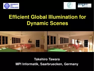
Efficient Global Illumination for Dynamic Scenes Takehiro Tawara MPI Informatik, Saarbruecken, Germany
Problem Statement • In the traditional rendering algorithms, every frame is considered separately. • The temporal coherence is poorly exploited • Redundant computations • The visual sensitivity to temporal detail cannot be properly accounted for • Too conservative stopping conditions • Temporal aliasing
Outline • Related Work • Background • Temporally-coherent Rendering Techniques: • Static Scenes (Walkthroughs) • Ray Tracing & IBR • Dynamic Scenes • Mesh-based Density Estimation • Photon Mapping, Final Gathering & Irradiance Cache • Efficient Handling of Strong Secondary Lighting • Conclusions
Related Work • Range-image framework: • Nimeroff et al. ’96 • Density Estimation • Dmitiriev et al. ’02 • Bi-Directional Path Tracing • Havran et al. ’03 • Perception-based / RADIANCE: • Yee and Pattanaik ’01 • Stochastic Ray Tracing • Meyer and Anderson ’06 • Progressive radiosity: • Chen’90, George et al. ’90, • Hierarchical radiosity: • Pueyo et al. ’97, Drettakis and Sillion ’97, Schöffel and Pomi ’99, • Instant radiosity: • Keller ’97 • Space-time hierarchical radiosity: • Damez ’99, Martin et al. ’03 • Global Monte Carlo radiosity: • Besuievsky and Sbert ’01
Background • 3D Warping and Pixel Flow • Density Estimation Particle Tracing • Photon Mapping • Animation Quality Metric (AQM)
Overview • Animation rendering solution: a hybrid of standard ray tracing and Image-Based Rendering (IBR) techniques. • Use ray tracing to compute all key frames and selected glossy and transparent objects. • For inbetween frames, derive as many pixels as possible using computationally inexpensive IBR techniques. • Animation quality enhancement: spatio-temporal antialiasing solution.
Selected case study scenes • Interesting occlusion relationships between objects which are challenging for IBR. • Many specular objects for the atriumscene. • Animation path causing great variations of the pixel flow for the room scene.
In-between frame generation MakeInbetweenFrames(k0,k2N) • kN’ = 3DWarp(k0) kN” = 3DWarp(k2N); • Mask out pixels: low PF, bad specular, IBR occlusion • if (AQM(kN’, kN”) > t) MakeInbetweenFrames(k0, kN) MakeInbetweenFrames(kN, k2N) • Else For(k1 to k2N-1) Composite(k0, k2N)
IBR-derived pixels to be ray traced • Pixels representing specular objects selected by the AQM predictions for recomputation. • Pixels with occlusion problems inherent to IBR techniques. • Pixels for slowly moving visual patterns, which are selected based on the Pixel Flow magnitude. The threshold velocity was found experimentally using subjective and objective (AQM) judgement of the resulting animation quality. • Totally, less than a half percentage of pixels is computed by ray tracing (Atrium: 49.5 %, Room: 35.1%).
Spatio-temporal antialiasing • 3D low-pass filtering in the spatio-temporal domain is performed as a post-process on the complete animation sequence. • Motion-compensated filtering is performed in the temporal domain (this is another application of the Pixel Flow derived as a by-product of IBR computations). • To our experience, for moving visual patterns a single ray-traced sample per pixel is enough to produce an animation which is visually indistinguishable from its counterpart based on supersampled images.
Examples of final frames Adaptively Supersampled frame used in traditional animations Corresponding frame derived using our approach In both cases the perceived quality of animation seems to be similar! Speedup x8.3
Perception-Guided Global Illumination Solution for Animation Rendering
Focus • Indirect lighting in animated sequences • Quite costly to compute • Usually changes slowly and smoothly both in the temporal and spatial domains
Temporal photon processing: contradictory requirement • Maximize the number of photons collected in the temporal domain to reduce the stochastic noise. • Minimize the time interval in which the photons were traced to avoid collecting invalid photons. Moving object Static object
Temporal photon processing: our solution • Energy-based stochastic error metric • Decides the number of frames to collect photons in temporal domain • Computed for each mesh element and for all frames • We assume that hitting a mesh element by photons can be modeled by the Poisson distribution. • Perception-based animation quality metric • Decides the number of photons per frame • Computed once per animation segment
Algorithm • Initialization: determine the initial number of photons per frame. • Adjust the animation segment length depending on temporal variations of indirect lighting which are measured using energy-based criteria. • Adjust the number of photons per frame based on the AQM response to limit the perceivable noise. • Spatio-temporal reconstruction of indirect lighting. • Spatial filtering step.
Temporal processing Off 25,000 photons/frame On 10,000-40,000 photons/frame
Timings [seconds] Timings of the indirect lighting computation for a single frame obtained as the average cost per frame for the whole animation (800 MHz Pentium III processor).
Localizing the Final Gathering for Dynamic Scenes using the Photon Map
Indirect Illumination Li • We separate the computation of Li as a function of dynamic changes in lighting: • Rapidly changingindirect illumination Ly: • Computed for scene regions strongly affected by dynamic objects, • Exact computation repeated for each frame. • Slowly changingindirect illumination Lt: • Computed for the remaining scene regions, • Reused information for an animation segment with more relaxed update of dynamic lighting component for each frame.
Photon Maps • We store photons into: • Static photon map • Estimate illumination when dynamic objects are removed from the scene, • Computed once per animation segment. • Global photon map (commonly used) • Estimate illumination for the complete scene, • Computed for each frame. • Dynamic photon map • Estimate the indirect illumination contributed only from dynamic objects, • Computed for each frame.
Tracing Dynamic Photons • Dynamic photon map is built simultaneously with the global photon map • It stores only the so-called dynamic photons which intersect with dynamic objects at least once. • The photon hit points are stored for diffuse surfaces only. • Photons with negative energy are possible in the regions occluded by dynamic objects. Dynamic objects
Static and Dynamic Irradiance Caches • Static irradiance cache is based on the static photon map • Computed only once for an animation segment, • Cache positions are the same for all frames, • Updated for each frame using the dynamic photon map • Used to compute Lt • Dynamic irradiance cache is computed using the global photon map for the current frame • Recomputed for each frame for selected regions • Used to compute Ly Static irradiance cache Dynamic irradiance cache
Determining Lyand Lt Scene Regions • Influence I of dynamic objects is computed using the dynamic photon map: • Indirect illumination Li:
Full global illumination Lr Influence I Rapidly changing indirect illuminationLy Slowly changing indirect illuminationLt
Animation Rapidly changing indirect illuminationLy Full global illumination Lr
Results • Our method • Recomputes 3 - 4 times less irradiance samples per frame, • Speeds up the computation 1.4 - 3.2 in respect to the frame-by-frame approach, • Improves the overall animation quality by reducing the flickering of reconstructed indirect lighting.
Exploiting Temporal Coherence in Final Gathering for Dynamic Scenes
Motivation • Final gathering is necessary to render a high quality global illumination animation. • For a dynamic environment, final gathering is repeated from scratch for every frame. • A long computation time • Stochastic noise can be easily perceivedin an animation. • To solve the both problems, we exploit temporal coherence. • We store incoming radiance samples and their information is shared for the neighboring animation frames.
Cache Data Structure • At each cache location 200 – 1,000 directions are sampled. • For each direction, incoming radiance, distance to the nearest intersection point and a flag are stored (total 8 bytes). • Cache locations are kept in memory as a kd-tree structure and sampled incoming data is stored in a hard disk. struct IncomingRadianceSample { RGBE Li; float16 Di; ushort flag; };
Temporally Coherent Gathering:Random Permutation with Non-uniform Probabilities This image illustrates our temporally coherent gathering algorithm for three frames. The grid depicts 16 stratified sampling directions in the upper hemisphere over a cache location. The lower row shows the corresponding cumulative distribution function (CDF) which is used to select a sampling direction. • A random integer X [0, T) is mapped to the corresponding cell. • After the selected cell (the shaded area) is removed, a new CDF (the bold dashed line) is rebuilt.
The Number of Refreshing Rays • Fixed number (e.g. 10% of the gathering rays) • Statistically all cells should be refreshed after 10 frames. • About 10 times faster computation • Adaptive number based on the number of gathering rays hitting on dynamic objects Reference Fixed Adaptive
Cache Locations • A new cache will be automatically inserted. • Examine redundancy by the nearest neighbor search. Without removing the redundant caches Removing the redundant caches
Moving a Light Source Full Indirect Speedup x5.2 for indirect illumination
Frame-by-frame Our method Speedup x9.1 for indirect illumination
Distribution of Incoming Radiance Samples over the Hemisphere a) b) a) Frame-by-frame computation b) 10 % of samples is refreshed for each frame according to the agingcriterion Correspondence of Irradiance
Efficient Rendering of Strong Secondary Lighting in Photon Mapping Algorithm
Noise Reduction Techniques • Variance reduction techniques • Stratified sampling • Importance sampling • Separation of an integrand • Importance sampling based on a BRDF • Easy for glossy surfaces • Difficult for diffuse surfaces
Overview • Global grid structure • Split a global photon map into: • Low-energy photon map • Stratified sampling • High-energy photon map • Explicit sampling toward bright regions
Algorithm • Global grid, in which each voxel has a counter which is the number of photons hitting on a surface in the voxel. • During a photon tracing phase: • If (counter <=cmax) • The photon is stored in a low-energy photon map. • If (counter >cmax) • The photon is stored in a high-energy photon map.
High-Energy Photon Map • Distribution of photon hit points in the high-energy photon map. • The black dots in the upper left region around the primary light source represent photons from this map.
Reflected Radiance Lh • Lh: Reflected radiance for a high-energy photon map • M: Set of brighter voxels • f: BRDF • V: Visibility function (1: visible, 0: otherwise) • dEh: Differential irradiance from a voxel
Scene 1 • Size: 320 x 240 pixels • a) 768 stratified samples / pixel • Rendering time: 21 min. • b) 278 samples / pixel • 48 stratified samples • 230 explicit samples • Rendering time: 9 min. a) b)
Scene 2 • Size: 1,128 x 480 pixels • 398 samples / cache • 300 stratified samples • 98 explicit samples • 13,666 caches • Rendering time: 10 min.
Conclusions • We presented a number of global illumination algorithms that exploit temporal coherence in lighting distribution for subsequent frames to improve the computation performance and overall animation quality. • Our strategy relied on extending into temporal domain global illumination and rendering techniques such as density estimation path tracing, photon mapping, ray tracing, and irradiance caching, which were originally designed to handle static scenes only. • Our solutions led to significant improvements of the computation performance and animation quality through the suppression of temporal aliasing.
Results: Statistics and Timings Specular pixels 40.8% Slow motion 2.4% IBR occlusions 0.3% Keyframes 6.0% -------------------------------- Total 49.5% Atrium Room Slow motion 28.1% IBR occlusions 1.9% Keyframes 5.1% ------------------------------ Total 35.1% Percentage of pixels to ray trace Average computation time / frame
Results: photon collection for each mesh element Fixed Adaptive Pixels with the AQM predicted perceivable differences [%] Number of frames in an animation segment