Half-Space Intersections
This paper explores an innovative randomized algorithm for determining the intersection of n half-planes in 2D and extends the analysis to 3D, resulting in a convex polyhedron represented as a graph. We outline the algorithm's mechanics, including the management of vertices during half-space additions and deletions, ensuring constant time complexity for certain operations. Furthermore, the expected run time of our method is analyzed, demonstrating an overall performance of O(n log n) for both half-space intersection and the 3D convex hull problem.

Half-Space Intersections
E N D
Presentation Transcript
Half-Space Intersections Randomized algorithm and expected run time analysis
Problem Definition – 2D • Given n half-planes as linear inequalities, we wish to find a boundary where they all intersect
Problem Definition – 3D • We extend our problem to 3D • The intersection is a convex polyhedron • This polyhedron is represented as a graph with degree 3 • inter(S): the intersection of a set S of half-spaces http://wpcontent.answers.com/wikipedia/commons/thumb/6/65/Half_Space.svg/300px-Half_Space.svg.png
Further Assumptions • inter(S) is bounded. If not – there’s a point at infinity which bounds it • No 3 vertices are collinear • Intersection of planes and spaces can be computed in constant time • Deciding if a point is inside a half-space can be computed in constant time
Algorithm Outline • Randomize a permutation of the set S of half spaces • For : • Add half space hito inter(Si-1) by • removing all the vertices in • adding new vertices on the boundary of
Addition of a Half Space • At step i we have a bidirectional pointer from every to some • When we add hi we start at the conflicting vertex and search the graph until we enter hi • We destroy all the vertices we encounter and create new ones on the face of
Pointer Update • Recall: the pointer is bidirectional • When we delete a vertex v pointing to a half-space h ∈ S \ Siwe have to find a new vertex w, such that • We perform BFS along until we encounter vertices inside inter(Si). This is our w.
Number of Vertices Created • Backwards analysis: suppose we delete vertices from inter(Si) and get inter(Si-1) • The convex polyhedron inter(Si) has i faces and O(i) vertices (because the degree is bounded by 3) • If we choose one of i half-spaces to delete, the expected number of vertices we delete is • Hence: the expected number of vertices created at the addition of hi is constant
Search Cost Analysis • When adding a half-space, we perform a BFS starting from the pointed vertex • Time – linear in # of deleted vertices • Each deleted vertex was created once: we only count creations • How many vertices are created in total?
Total # of Vertices Created • Total vertices created when adding hi: • c(H,h):# of conflict vertices between inter(H) and h • Backwards analysis – the expectation over all hi is bounded by: since the degree of each vertex is bounded by 3
Total # of Vertices Created • hi+1 is chosen randomly, so: • The expected # of vertices is bounded by: • We saw the algorithm runs in time linear to the number of vertices created, so this expression also bounds the run time of the algorithm
Bounding the Total Run Time • c(Si,hi+1) is also the expected number of vertices deleted by the addition of hi+1
Bounding the Total Run Time • Let tc(v) be the time v is created and td(v) be the time v is destroyed • Then: for all the vertices v created in the algorithm
Bounding the Total Run Time • Obviously, tc(v) ≤ td(v) – 1. Therefore: • Recall that the expected number of vertices created at each iteration is constant! Constant
Bounding the Total Run Time • The total run time of the algorithm is:
Convex Hull in 3D • Using duality we can reduce the problem of convex hull in 3D to finding half-space intersection (in 3D) • We just saw how to compute the half-space intersection in O(nlogn) time • 3D Convex Hull problem takes also O(nlogn) time to compute