Principal component regression
220 likes | 461 Vues
Principal component regression. When simple linear model fails Ridge regression Lasso Principal component analysis Principal component regression . When parameters are highly correlated.

Principal component regression
E N D
Presentation Transcript
Principal component regression When simple linear model fails Ridge regression Lasso Principal component analysis Principal component regression
When parameters are highly correlated There are many situations when simple linear models fail to give satisfactory results. One class of cases where it happens when the rank of the input (design) matrix is less than the number of parameters or even worse when condition number (ratio of smallest eigenvalue to the largest) of the matrix XTX is very small. These situations may cause problem in model selection. In simple cases we removed one parameter after another (eliminated variables) and did tests using various techniques (t-test, AIC/BIC, cross validation). This approach is good when we want to select few parameters out of many to design our predictions. It could be used when we want to know which of the input variables are relevant for prediction. However in many cases removing some of the parameters may not have physical meaning. It may happen when input matrix is highly correlated or the number of input parameters is larger than the number of observations or we know that all input parameters are relevant. There are several approaches to this type of problems. Examples are ridge regression, lasso, principal component regression, partial least squares, Bayesian estimation. We will not consider partial least-squares and Bayesian estimation.
Ridge regression Let us say we have input (X) variables and response y. We want to estimate linear relationship between input and response: Ridge regression is a simple modification of least-squares approach. In this approach diagonal of XTX matrix is modified to make sure that the matrix is well conditioned In this case effective number of parameters is calculated using ke=tr(X(XTX+λI)-1XT)=tr((XTX+λI)-1XTX). This value is used in model selection using BIC or AIC calculations. No the value of ke is also part of the model. Model selection could be done using AIC/BIC or cross-validation. There is an R command for ridge regression: lm.ridge
Lasso As it can be seen one interpretation of ridge regression is to find parameters of the system and make sure that L2 norm does not become very large. A modification of this is known as LASSO method: Find parameters of the model using least-squares under condition that the L1 norm of the parameter vector does not become very large. Parameter c can be found using cross validation. Here it is not clear how to calculate the effective number of freedom. Using BIC or AIC would be difficult. I could not find R command for lasso.
Purpose of PCA The main idea behind the principal component analysis is to represent multidimensional data with fewer number of variables retaining main features of the data. It is inevitable that by reducing dimensionality some features of the data will be lost. It is hoped that these lost features are comparable with the “noise” and they do not tell much about underlying population. The method PCA tries to project multidimensional data to a lower dimensional space retaining as much as possible variability of the data. This technique is widely used in many areas of applied statistics. It is natural since interpretation and visualisation in a fewer dimensional space is easier than in many dimensional space. Especially if we can reduce dimensionality to two or three then we can use various plots and try to find some structure in the data. Principal components can also be used as a part of other analysis (modeling, regression, feature selection, clusterisation). Its simplicity makes it very popular. But care should be taken in applications. First it should be analysed if this technique can be applied. For example if data are circular then it might not be wise to use PCA. Then transformation of the data might be necessary before applying PCA. PCA is one of the techniques used for dimension reductions.
Covariance and Correlation matrices Suppose we havean nxp data matrix X: Where rows represent observations and columns represent variables. Without loss of generality we will assume that column totals are 0. If it would not be the case then we could calculate column averages and subtract then from corresponding column. Covariance matrix is calculated using (when column averages are 0): Correlation matrix is calculated using: I.e. by normalisation of covariance matrix by its diagonals. Both these matrices are symmetric and non-negative.
Principal components as a linear combination of the original parameters Let us assume that we have a random vector x with p elements (variables). We want to find a linear combination of these variables so that variance of the new variable is large. I.e. we want to find new vector y: so that it has maximum possible variance. It means that this variable contains maximum possible variability of the original variables. Without loss of generality we can assume that mean values of the original variables are 0. Then for variance of y we can write: Thus the problem reduces to finding maximum of this quadratic form. If found, this new variable will be the first principal component.
PCA using eigenvalues We can write the above problem in a matrix-vector form: But by multiplying to a scalar value this expression (quadratic form) can be made as large as desired. Then we require that length of the vector is unit. I.e. desired vector is on the unit sphere (p-dimensional) that satisfies the condition: Now if we use Lagrange multipliers technique then it reduces to unconditional maximisation of: If we get derivative of the left side and equate to 0 we have: Thus the problem of finding unit length vector with largest variance reduces to finding the largest eigenvalue and corresponding eogenvector. If we have largest eigenvalue and corresponding eigenvector then we can find the second largest eigenvalue and so on. Finding principal components is equivalent to finding all egienvalues and eigenvectors of the matrix S.
PCA and eigenvalues/eigenvectors Note that since matrix S is symmetric and non-negative definite all eigenvalues are non-negative and eigenvectors are orthonormal (v-s are the eigenvectors). I.e.: vi-s contain coefficients of principal components. They are known as factor loadings. The var(vix)=iholds, i.e variance of the i-th component is the i-th eigenvalue. First principal component accounts the largest amount of the variance in the data. Xvi gives scores of the n individuals (observation vectors) on this principal component. Relation: shows that sum of the eigenvalues is equal to the total variance in the data. Where is the diagonal formed by the eigenvalues and V is the matrix formed by the eigenvectors of the covariance (correlation) matrix. Columns of this matrix is called loadings of principal components that is the amount of each variable’s contribution to the principal component. When the correlation matrix is used then the total variance is equal to the dimension of the original variables, that is p. Variance of i-th principal component is i. It is often said that this components accounts i/jj proportion of the total variance. Plotting the first few principal components together with observations may show some structure in the data.
PCA using SVD Since we know that principal component analysis is related with eigenvalue analysis we can use similar techniques available in linear algebra. Suppose that X is mean centered data matrix. Then we can avoid calculating covariance matrix by using singular value decomposition. If we have the matrix nxp we can use SVD: where U is nxnV is pxp orthogonal matrices. D is nxp matrix. p diagonal elements contains square root of the eigenvalues of XTX and all other elements are 0. Rows of V contains coefficients of the principal components. T=UD contains scores of the principal components that is the amount of each observation’s contribution to the principal components. Some statistical packages use eigenvalues for principal component analysis and some use SVD.
Scaling It is often the case that different variables have completely different scaling. For examples one of the variables may have been measured in meters and another one in centimeters (by design or accident). Eigenvalues of the matrix is scale dependent. If we would multiply one column of the data matrix X by some scale factor (say s) then variance of this variable would increase by s2 and this variable can dominate whole covariance matrix and hence the whole eigenvalue and eigenvectors. It is necessary to take precautions when dealing with the data. If it is possible to bring all data to the same scale using some underlying physical properties then it should be done. If the scale of the data is unknown then it is better to use correlation matrix instead of the covariance matrix. It is in general recommended option in many statistical packages. It should be noted that since scale affects eigenvalues and eigenvectors then interpretation of the principal components derived by these two methods can be completely different. In real life applications care should be taken when using correlation matrix. Outliers in the observation can affect covariance and hence correlation matrix. It is recommended to use robust estimation for covariances (in a simple case by rejecting of outliers). When using robust estimates covariance matrix may not be non-negative and some eigenvalues might be negative. In many applications it is not important since we are interested in the principal components corresponding to the largest eigenvalues. Standard packages allow using covariance as well as correlation matrices. R allows input the data, the correlation or the covariance matrices.
Screeplot Scree plot is the plot of the eigenvalues (or variances of principal components) against their indices. For example plot given by R. When you see type of plot similar to that on the left with one dominant eigenvalue (variance) then you should consider scaling. Scree plot with covariance matrix Scree plot with correlation matrix
Dimension selection There are many recommendations for the selection of dimension. Few of them are: • The proportion of variances. If the first two components account for 70%-90% or more of the total variance then further components might be irrelevant (NB: problem with scaling) • Components below certain level can be rejected. If components have been calculated using a correlation matrix, often those components with variance less than 1 are rejected. It might be dangerous. Especially if one variable (if a covariance matrix is used) is almost independent of others then it might give rise the component with variance less than 1. It does not mean that it is uninformative. • If the uncertainty (usually expressed as standard deviation) of the observations is known, then components with variances less than that, certainly can be rejected. • Scree plot: If scree plots show elbow then components with variances less than this elbow can be rejected. • There is cross-validation technique. One value of the observation is removed (xj) then using principal components this value is predicted and it is done for all data points. If adding the component does not improve prediction power then this component can be rejected. This technique is computer intensive (NB: problem with outliers). Prediction error calculated using: It is PREdiction Sum of Squares and is calculated using first m principal components. If this value is 1 (some authors recommend 0.9) then only m-1 components are selected.
Biplots Biplots are useful way of displaying the whole data in a fewer dimensional space. It is the projection of observation vectors and variables to k<p dimensional space. How does it work? Let us consider PCA with SVD If we want a twi dimensional biplot then we equate all elements of the D to 0 but the first two. Denote it by D*. Now we have the reduced rank representation of X: Now we want to find GHT representation of the data matrix where the rows of G and the columns of HT are scores of the rows and the columns of the data matrix. We can choose them using: The rows of Gand H are then plotted in biplot. It is usual to take =1. In this case G and H are scores of observations on and contribution of variables to principal components. It is considered to be most natural biplot. When =0 then vector lengths corresponding to the original variables are approximately equal to their standard deviations.
Biplots Biplots show: • Standard deviation of variables • Value of observations on variables • Correlation between variables • Relative positions of observations in few dimensional spac It can be used to identify clusters if there is any, outliers, relation between variables and relevance of the observations to the variables
Biplots: example USArrests data. The result of princomp with correlation matrix. It is clear that three variables are close to each other and correlation between them is higher. UrbanPop is has less correation with these variables. There seems to be some clusters in the data.
Principal component regression Principal component regression combines ideas behind principal components analysis and regression analysis. In this approach the first step is calculation of principal components. Let us say (again) that we have input matrix – X and response variable y. We can use singular value decomposition of X Let us say the number of input variables (then number of columns in X matrix) is m and we want to use only p variables. Then we do Now we define score matrix as (D* is a diagonal matrix of modified singular values): Now we can use T as input matrix (it has p columns, i.e. p variables). Now we can estimate parameters using: New parameters – α are linearly related with old parameters – β = Vα. Once we have parameters using principal component regression we can calculate the values for the original parameters.
Principal component regression One of the problems of principal component regression is how to select the number of dimensions (variables). There are several appraoches: • Proportion of variance explained. This approach is based only on input parameter space and may not be useful for wide range of problems • Cross validation. How many components can predict output without adding unstabity • AIC/BIC
R commands for PCA First decide what data matrix we have and prepare that matrix. Necessary commands for principal component analysis are in the package called mva (in newer version it is in stats package). This package contains many functions for multivariate analysis. First load this package using library(mva) – loads the library mva data(USArrests) – loads data pc1 = princomp(data,cor=TRUE) - It does actual calculations. if cor is absent then PCA is done with covariance matrix. summary(pc1) - gives standard deviations and proportion of variances pc1$scores -gives scores of the observation vectors on principal components pc1$loadings screeplot(pc1) - gives scree plot. It plots the values of eigenvectors vs their number biplot(pc1) – gives biplot. It would be recommended to use correlation and for quick decision use biplot
R commands for PCR Commands for principal component regression are in the package pls install.packages(‘pls’) # You need to do it only once library(pls) # You need to do it every time you start R session yarn.pcr <- pcr(density ~ NIR, 6, data = yarn, validation = "CV") plot(yarn.pcr$validation$PRESS[1,])
References • Krzanowski WJ and Marriout FHC. (1994) Multivariate analysis. Vol 1. Kendall’s library of statistics • Rencher AC (1995) Methods of multivariate analysis • Mardia,KV, Kent, JT and Bibby, JM (2003) Multivariate analysis • Jollife, IT. (1986) Principal Component Analysis