Download
1 / 125
1.43k likes | 2.16k Vues
Switching and Routing. Foreleser: Carsten Griwodz Email: griff@ifi.uio.no. company. ISP. Motivation. one frame at a time, Min 512 bits. It is desirable to connect networks (instead of using a single large one): Limits in physical size and number of nodes per network

E N D
Switching and Routing Foreleser: Carsten Griwodz Email: griff@ifi.uio.no 1
company ISP Motivation one frame at a time, Min 512 bits • It is desirable to connect networks (instead of using a single large one): • Limits in physical size and number of nodes per network • Limits in amount of concurrent traffic per network • Different kinds of network for different needs • Separate networks for increased availability • Administrative boundaries wireless network Max 500m
Connecting Networks by Relays End system Intermediate system End system 5 5 Application layer Gateway 4 4 Transport layer 3 Router 3 Network layer 2 Bridge 2 Data link layer 1 Repeater 1 Physical layer
Layer 1: Repeater / Hub copies all bits between cable segments works solely as a repeater does not influence the traffic between networks Layer 2: Bridge / Switch relays frames between LANs (MAC level) minor frame modifications, increases the number of stations Layer 3: Router (or Layer 3 Gateway) relays packets between different networks modifies the packets converts different addressing concepts Layer 4 - 5: Gateway (or Protocol Converter) converts one protocol into another usually no 1-to-1 mapping of functions Connecting Networks by Relays • Note: • names (in products) are often confused • e. g. bridge and switch
Repeater and Hub Hub ex.: IEEE 802.3 Twisted Pair Repeater ex.: IEEE 802.3 “Thinwire” • Function • To amplify the electrical signals • To increase the range • Limitation • Extends the broadcast medium: every bit is copied • One collision domain
Bridges, Switches • Bridges • Connects two or more LANs (potentially different types) • Each line is its own collision domain • Traditionally: store-and-forward and CPU-based • Switches • Typically connects two or more computers • Each port / line is its own collision domain (no collisions) • Typically cut-through switching devices • begin forwarding as soon as possible • when destination header has been detected, before rest of frame arrived • Hardware-based • Bridges vs. Switches • Sometimes difference seems to be more a marketing issue than technical one
Bridge • Tasks • Coupling of different LANs • Scalability of networks • To increase capacity • To increase reliability • To improve security • To cover large distances • To offer independence from protocols • IP OSI layer 2 protocols • Ethernet versions • Important goal: to achieve transparency • Change attachment point without changes to HW, SW, configuration • Hide different types of LAN to communicating machines
Bridge Connecting 2 Different Networks Example: Bridge between IEEE 802.3 (CSMA/CD) and IEEE 802.4 (Token Bus) • Approach • LLC as common layer • Frames are routed to the respective MAC • Bridge contains • Its own implementation for each MAC • For each to it belonging physical layer the corresponding implementation
802.x 802.y Bridging • Some different 802.x frame formats: • There are even more different frame formats ... • Some fields are technically necessary in one case but useless in another • e.g. duration of 802.11
802.x 802.y Bridging • Different transmission rates (4/10/11/16/100/1000/... Mbps) • Bridge between fast LAN and slow LAN (or several LANs to one) • Buffering frames which cannot be transmitted immediately • Potentially many frames must be buffered within bridge • If bridge is out of memory, frames are dropped • Different frame lengths • 802.3: 1518 bytes, 802.4: 8191 bytes, 802.5: unlimited, 802.11: 2346 bytes • 802.x protocols do not support reassembly • Bridge must not segment frames that are too large • Frames that are too long are dropped • Implies a loss of transparency • Special case 802.6 – DQDB transmits each frame in several cells • Different features • Priorities • Supported (in various forms) from both 802.4 and 802.5 • Not supported by 802.3
802.x 802.y Bridging • Different checksum calculations • Means conversion, delay, buffering • Security • 802.11 provides some data link layer encryption • 802.3 does not • Quality of Service / Priorities • Supported (in various forms) by both 802.4 and 802.5 • Not supported by 802.3 • ’Kind of’ in 802.11 (PCF / DCF) • Acknowledgements • Supported by 802.4 (temporary token handoff) • Supported by 802.5 (C+A bits) • Not supported by 802.3
address LAN A 1 B 2 C 2 D 2 Self–Learning Bridges • Also called Transparent Bridges • Transparency • Bridges not visible for the other components of the network simplifies other components • Transparent bridge • Bridge works in promiscuous mode(receives every frame of each connected LAN) • Bridge manages table: station LAN(output line) • Decision procedure • Destination unknown: flooding • Source and destination LANs identical: frame dropped • Source and destination LANs differ: frame rerouted to destination LAN
Self–Learning Bridges • Learning procedure • Bridge table initially empty • Use flooding for unknown destination • Backward learning • Bridge works in promiscuous mode: • Receives any frame on any of its LANs • Bridge receives frames from source address Q on LAN L • Q can be reached over L • Create table entry accordingly • Adaptation to changes in topology • Entry associated with timestamp (last frame arrival time) • Timestamp of an entry (Z, LAN, TS) is updated when frame received from Z • Entries that are not updated are purged
Self–Learning Bridges: Spanning Tree • Increase reliability • Connect LANs via various bridges in parallel • Problem • This creates a loop in the topology • Frames with unknown destination are flooded • Frame is copied again and again • Solution • Communication among bridges • Overlay actual topology by spanning tree reaching every LAN • Exactly one path from any LAN to every other LAN
Self–Learning Bridges: Spanning Tree • Algorithm • Choose a bridge as root of tree • All bridges broadcast their serial number, lowest wins • Generation of spanning tree • Configured with bridges representing the edges within the tree • Thereby avoiding loops • Adaptation if configuration is changed • Drawback • Ignores some potential connections between LANsi.e., not all bridges are necessarily present in the tree
Source Routing Bridges • Alternative to self-learning bridges • Principle • The frame’s sender defines path • Bridge routes the frame • Prerequisite • LAN has a unique address • Bridge at the respective LAN is also unique • Then • Sender flags the frame (top bit of its own address = 1),if destination address is not reachable in LAN • Bridge routes only frames that have been flagged in such a way • Determining Path • Sender sends discovery frames as broadcast • Each bridge forwards on all attached LANs • Each bridge on the path adds own address to return packet • Problem: high traffic
Connecting Equal Networks: Encapsulation Example: remote bridge • Principle • Incoming data unit is packaged as payload, • Transmitted and • Then fed into the destination network • Properties • Certain protocol on connecting route • e.g. PPPi.e. MAC frames encapsulated in PPP • Only bridge at the destination network can be reached • Simple
Intermediate systems End systems Subnetworks Network Layer • Goal • Enable data transfer fromend system to end system • Several hops, (heterogeneous) subnetworks • Compensate for differences between end systems during transmission • The provided services are • Standardized for end systems • Independent from network technology • Independent from number, type and topology of the subnetworks • Subnetworks (ISO definition): • A multiple of one or several intermediary systems that provide switching functionalities and through which open end systems can establish network connections • Routers are such Intermediate Systems
Network Layer • Primary task from a layer model perspective • To provide service to the transport layer • Connectionless or connection-oriented service • Uniform addressing • Internetworking: provide transitions between networks • Routing • Congestion control • Quality of Service (QoS)
Inside: Types of Switching • Circuit switching • Switching a physical connection • Packet switching • Store-and-forward, but transmissions packets limited in size • Message switching • Message is stored and passed one by one hop
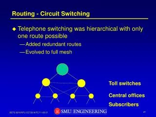
Circuit Switching • Connection exists physically for the duration of the conversation • Refers to • Switching centers • Connections between switching centers(frequency spectrum, dedicated ports) • Implementation examples • Historically: on switching boards • Mechanical positioning of the dialers • Setting coupling points in circuits
Packet Switching • Datagrams • Every packet chooses its path • Virtual circuits • Packets (or cells) over a pre-defined path
Packet Switching • Packets of limited size • Dynamic route search (no connect phase) • No dedicated path from source to destination
Message Switching • All data to be sent are treated as a "message" • “Store and forward" network • Accept • Treat of possible errors • Store • Forward
Comparison: Temporal Performance Circuit switching Message switching Packet switching Virtual circuit
Comparison: Properties • Circuit switching • Connection has to occur before transmission • Establishing a connection takes time • Resource allocation too rigid (possibly waste of resources) • Once connection is established it cannot be blocked anymore • Packet switching • Possibly only reservation of average bandwidth (static reservation) • Possibility of congestion • High utilization of resources • Message switching • High memory requirements at the node (switching centers) • Node may be used to its full capacity over a longer period of time by one message
Circuit switching Connection establishment can take a long time Bandwidth is reserved No danger of congestion Possibly poor bandwidth utilization (burst traffic) Continuous transmission time all data is transmitted over the same path Packet switching Connect phase not absolutely necessary Dynamic allocation of bandwidth Danger of congestion Optimized bandwidth utilization Varying transmission time packets between same end systems may use different paths Comparison: Circuit and Packet Switching
Virtual Circuits • Connection set-up phase • Select a path • Intermediate systems store path information • Network reserves all resources required for the connection • Data transfer phase • All packets follow the selected path • Packet contains VC’s number • Identification of connection, no address information • IS uses the stored path information to determine the successor • Disconnect phase • Network forgets the path • Releases reserved resources
Implementation Virtual Circuit End systems ES allocate VC-numbers independently Problem: the same VC-identifiers may be allocated to different paths • Solution: allocate VC-numbers for virtual circuit segments • IS differentiates between incoming and outgoing VC-number • IS receives incoming VC-number when connect request arrives • IS creates outgoing VC-number (unique between IS and successor(IS)) • IS sends outgoing VC-number in connect request
A 0 C 0 H 0 C 1 H 1 A 0 B 0 D 0 A 1 F 0 B 1 D 1 H 2 F 1 E 0 H 0 F 0 H 0 E 1 D 2 H 0 B 0 H 1 E 0 C 0 H 0 B 0 E 1 C 1 H 1 H 2 B 1 F 0 H 2 H 3 E 2 F 1 H 3 H 4 E 3 C 2 F 0 A 0 F 0 E 0 D 0 A 1 H 0 B 0 D 1 A 2 C 0 B 1 H 0 A 3 C 1 D 0 B 0 Implementation Virtual Circuit B C A IN OUT D 8 Simplex virtual circuits E F 0 - ABCD 0 - BCD 1 - AEFD 1 - BAE 2 - ABFD 2 - BF 3 - AEC 4 - AECDFB
Implementation Datagram • Datagram passes through the network as an isolated unit • Has complete source and destination addresses • Individual route selection for each datagram • Generally no resource reservation • Correct sequence not guaranteed
Datagram: IS routing table specifies possible path(s) No connection setup delay Less sensible to IS and link failures Route selection for each datagram: quick reaction to failures but Each packet contains the full destination and source address Route selection for each datagram: overhead QoS guarantees hardly possible Virtual Circuit: destination address defined by connection Packets contain short VC-number only Low overhead during transfer phase “Perfect" channel throughout the net Resource reservation: "Quality of Service" guarantees possible but Overhead for connection setup Memory for VC tables and state information needed in every IS Sensible to IS and link failures Resource reservation: potentially poor utilization Datagram vs. Virtual Circuit
Services of the Network Layer • Concepts • Connection oriented vs. connectionless communication • Connection oriented • Error free communication channel • Usually error control, flow control, ... • Usually duplex communication • More favorable for real-time communications • Favored by telephone and telecommunication companies • Connectionless • Unreliable communication • Hardly any error control: left to layer 4 or higher • Simplex communication • More favorable for simple data communication: • Favored by Internet community
Connection Oriented Communication • Connection Oriented Communication • 3-phase interaction • Connect • Data transfer • Disconnect • (allows for) Quality of Service Negotiation • (typically) Reliable Communication in both directions • Flow Control • Relatively complex protocols • Connection-Oriented Service • Service provider offers • Queues in both directions • Ordered transmission of objects • Delivery of objects at most once
Connectless communication • Connectionless Communication • Network transmits packets as isolated Units (datagram) • Unreliable Communication • loss, duplication, modification, sequence errors possible • No flow control • Comparatively simple protocols • Connectionless Service • Service provider can • Delete objects in a queue • Duplicate objects in a queue • Change the object sequence within a queue
Arguments pro a connection oriented service Simple, powerful paradigm Simplification of the higher layers Relieves end systems For some applications efficiency in time is more important than error-free transmission e. g. real-time applications, digital voice transmission) suitable for a wide range of applications Arguments pro a connectionless service High flexibility and low complexity Costs for connects and disconnects are high for transaction oriented applications Easier to optimize the network load Compatibility and costs IP common, can’t change now ‘End-to-End Arguments’ secure communication requires error control within the application but error control in one layer can replace the error control in the layer underneath it Comparison of Concepts
Routing 42
Routing: Foundations • Task • To define the route of packets through the network • From the source • To the destination system • Routing algorithm • Defines on which outgoing line an incoming packet will be transmitted • Route determination • Datagram • Routing algorithm makes individual decision for each packet • Virtual circuit • Routing algorithm runs only during connect (session routing)
desti- nation link A 0 B 3 C 1 D 4 Data packets Incoming lines Outgoing lines Routing: Routing and Forwarding • Distinction can be made • Routing: makes decision which route to use • Forwarding: what happens when a packet arrives Topology, link utilization, etc. information Router Routing Process Routing table Fills & Updates Uses & Looks up Forwarding Process
Good Properties for Routing Algorithms • Correctness • Simplicity • Minimize load of routers • Robustness • Compensation for IS and link failures • Handling of topology and traffic changes • Stability • Consistent results • No volatile adaptations to new conditions • Fairness • Among different sources compared to each other • Optimality
Routing Algorithms: Conflicting Properties • Often conflicting: fairness and optimization • Some different optimization criteria • Average packet delay • Total throughput • Individual delay • Conflict • Example: • Communication among A A’, B B’, C C’ uses full capacity of horizontal line • Optimized throughput, but • No fairness for X and X’ • Tradeoff between fairness and optimization • Therefore often • Hop minimization per packet • It tends to reduce delays and decreases required bandwidth • Also tends to increase throughput
Classes of Routing Algorithms • Class Non-adaptive Algorithms • Current network state not taken into consideration • Assume average values • All routes are defined off-line before the network is put into operation • No change during operation (static routing) • With knowledge of the overall topology • Spanning tree • Flow-based routing • Without knowledge of the overall topology • Flooding • Class Adaptive Algorithms • Decisions are based on current network state • Measurements / estimates of the topology and the traffic volume • Further sub-classification into • Centralized algorithms • Isolated algorithms • Distributed algorithms
r1 r1 I J K r2’ Optimality Principle and Sink Tree • General statement about optimal routes • If router J is on optimal path from router I to router K • Then the optimal path from router J to router K uses the same route • Example: • r1: route from I to J • r2: route from J to K • If better route r2’ from J to Kwould exist • Then • Concatenation of r1 and r2’ would improve route from I to K • Set of optimal routes • From all sources • To a given destination form a tree rooted at the destination: Sink Tree
B C A D E G J F I N H K L O M Sink Tree Sink Tree for Destination B Subnet • Comments • Tree: no loops • Each optimal route is finite with bounded number of hops • Not necessarily unique • Other trees with same path lengths may exist • Goal of all routing algorithms • Discover and use the sink trees for all routers • Not realistic to use Sink Trees as real-life routing algorithm • Need complete information about topology • Sink Tree is only a benchmark for routing algorithms
Methodology & Metrics • Networks represented as graphs: • Node represents a router • Edge represents a communication line (link) • Compute the shortest path between a given pair of routers • Different metrics for path lengths can be used • Can lead to different results • Sometime even combined (but this leads to computational problems) • Metrics for the "ideal" route, e.g., a "short" route • Number of hops • Geographical distance • Bandwidth • Average data volume • Cost of communication • Delay in queues • ...