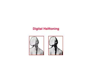
Digital Halftoning

1. Digital Halftoning

2. Summary of 30.1.06 lecture • How to produce illusion of the original tonal quality of a image by judicious placements of dots. • How to generate an image with fewer amplitude levels but perceptually similar to the original. • High frequency patterns are perceived as their macroscopic averages. • Halftoning techniques • Dithering • Disperse dot • Cluster dot • Error Diffusion • Floyd Steinberg Dithering mask Ξ screen

3. Dispersed masks • Print single ink dots; ability to deal with individual pixels of the image. Individual pixels are addressed. • M(i,j) is threshold mask • The numbers in the mask are so dispersed, that the black dots in the output are also well dispersed for each graylevel. • Problems • Stacking constraint – no solution

4. Periods of n& m can sometimes be detected • Solution: make nxm >> no. of distinct threshold elements, useful in blue noisemasks (low frequency attenuated) • Large nxm ; poor spatial resolution bigger mask: more gray levels. i.e Better gray/ dynamic range /colour resolution • Large masks are obtained using 2 smaller masks based on Thue-Morse sequence. • Clustered masks • They average over a neighborhood & replace by cluster of dots. Pixels in clustered dot are nucleated in groups in regular intervals. • Tradeoff between no.of gray levels to be rendered and size of cluster

5. Bigger cluster – more levels the mask can render – but more noticeable cluster in dither output • A method • Start with a larger mask consisting of several copies of a small mask with 256 levels (0-1) • For 0.5 gray level – checker board is ideal • Get versions of this checker board by a process of interpolation for intermediate gray levels • Trial & error & by judging output quality • A versatile method

6. Calibration of dither masks : In constructing dither masks, we assume that the no.of black pixels in a hlaftone pattern proportional to gray levels We call such - linear dither masks Will not work if there is dot overlap or dot gain Another point: Non linearity effect when a quantity called lightness is used to measure graylevels Lightness – perceived as log of luminance (how bright we see luminance) To compensate for this , apply a tone reproduction curve (TRC) to the input data & then use a linear dither mask.

8. Colour: • Use 4 different masks (screens) one for each color + black. using the same mask 4 times is usually avoided by the screens set at different angles. • Registration problem (moire pattren)

9. Error Diffusion: • Running error • Where at pixel location K, r(k) is a gray value number between 0 (w) – 1 (B) • ρ( k) = 0 for white = 1 for black • The running error satisfies the recursion

10. Simple error diffusion: • is defined by taking ρ(n+1) to satisfy the greedy algorithm. • i.e. ρ(n+1) takes the value 0 or 1 which ever minimizes Є (n+1), with a tie breaking rule (when error is exactly 0.5). • It can be shown that Є (n) lies in the interval [-1/2, 1/2] for any choice of the sequence Thus Є(n) is bounded and

11. 2 PAPERS

12. Minimum MSE output: result of a fixed threshold. The result of dithering with a white noise threshold.

13. CLUSTERED-DOT Result of halftoning with a 4x4 super-cell classical screen.

24. What is digital halftoning? • Digital halftoning is the process of rendering a continuous-tone image with a device that is capable of generating only two or a few levels of gray at each point on the device output surface. • The perception of additional levels of gray depends on a local average of the binary or multilevel texture.

25. The Two Fundamental Goalsof Digital Halftoning • Representation of Tone • smooth, homogeneous texture. • free from visible structure or contouring. Diamond dot screen Bayer screen Error diffusion

26. Modulation Strategies • Amplitude modulation - dot size varies, dot spacing is fixed. • Frequency modulation - dot spacing varies, dot size is fixed.

27. f f f Signal Spectra

28. Discrete Fourier Transform • A tool for measuring the frequency spectrum of signals. • For discrete time signals xn n=0,1, …, N-1.The Discrete Fourier transform (DFT) can be calculated byThe inverse Fourier transform calculates the time sequence from the frequency components: • Both the time sequence and the frequency components are complex numbers in general. The power spectral density of the time sequence x is

29. Application to Images • We need to define the concept of spatial frequency. This is the number of cycles measured per unit distance. low frequency high frequency

30. DC term Fundamental frequency Second harmonic Basis Set • Sinusoid is the basis for measuring spectral characteristics in the Fourier transform. Note that • The Fourier transform represents each signal sample as weighted average of sinusoids

31. Two Dimensional DFT • Straightforward extension of the 1-D DFT. • Equivalent to • taken 1-D DFT row by row • then take 1-D DFT of the result column by column column by column DFT row by row DFT

32. Human Visual Response • The human perception system do not have equal response to all spatial frequencies. • As the spatial frequencies become higher and higher, our ability to perceive the pattern will be lower and lower. • It turns out that our ability to perceive very low frequency patterns also decreases as the frequency decreases. • These characteristics can be captured using a contrast sensitivity function.

33. Contrast Sensitivity Function • [Mannos and Sakrison, 1974] fr Spatial frequency (cycles per degree perceived by the eyes)

34. Screening or Dithering Outline 1. Screening as a threshold process 2. Macroscreens 3. Spectral characteristics of screens

35. Threshold Screening is a Thresholding Process • Simple point-to-point transformation of each pixel in the continuous-tone image to a binary value. • Process requires no memory or neighborhood information.

36. Why Not Use a Single Threshold? • A single threshold yields only a silhouette representation of the image. • No gray levels intermediate to white or black are rendered. • To generate additional gray levels, the threshold must be dithered, i.e. perturbed about the constant value. Continuous-tone original image Result of applying a fixed threshold at midtone

37. Basic Structure of Screening Algorithm The threshold matrix is periodically tiled over the entire continuous-tone image.

38. Terminology • The screening process is also called dithering. • However, the term dithering is sometimes applied to any digital halftoning process, not just that consisting of a pixel-to-pixel comparision with thresholds in a matrix. • The following are equivalent terms for the threshold matrix: • screen • dither matrix • mask

39. How Tone is Rendered • If we threshold the screen against a constant gray value, we obtain the binary texture used to represent that constant level of absorptance.

40. Dot Profile Function • The family of binary textures used to render each level of constant tone is called the dot profile function. • There is a one-to-one relationship between the dot profile and the screen.

41. Selection of Threshold Values • For an MxN halftone cell,can print 0, 1, 2, …, MN dots, yielding average absorbances (occupancy ratio) 0, 1/MN, 2/MN, …, 1, respectively. • As the input gray level increases, each time a threshold is exceeded, we add a new dot, thereby increasing the rendered absorbance by 1/MN. • It follows that the threshold levels should be uniformly spaced over the range of gray values of the input image.

42. Rendering of Detail - Partial Dotting

43. Partial Dotting - Example

44. Spatial Arrangement of Thresholds • For clustered dot textures, thresholds that are close in value are located close together in the threshold matrix

45. Spatial Arrangement of Thresholds (cont.) • For dispersed dot textures, thresholds that are close in value are located far apart in the threshold matrix.

46. Detail Rendition with Dispersed Dot Screens • Compute the halftone image in the example given below to show how detail is rendered with a dispersed dot screen.

47. Detail Rendition with Dispersed Dot Screens • Solution

48. Clustered vs. Dispersed Dots • Note that these assessments are relative. • For example, at sufficiently high resolution, clustered dot textures will also have low visibility and good detail rendition.