Lecture 2: Learning without Over-learning
Lecture 2: Learning without Over-learning. Isabelle Guyon isabelle@clopinet.com. Machine Learning. Learning machines include : Linear discriminant (including Naïve Bayes) Kernel methods Neural networks Decision trees Learning is tuning: Parameters (weights w or a , threshold b)

Lecture 2: Learning without Over-learning
E N D
Presentation Transcript
Lecture 2:Learning withoutOver-learning Isabelle Guyon isabelle@clopinet.com
Machine Learning • Learning machines include: • Linear discriminant (including Naïve Bayes) • Kernel methods • Neural networks • Decision trees • Learning is tuning: • Parameters (weights w or a, threshold b) • Hyperparameters (basis functions, kernels, number of units)
Conventions n X={xij} y ={yj} m xi a w
What is a Risk Functional? • A function of the parameters of the learning machine, assessing how much it is expected to fail on a given task. R[f(x,w)] Parameter space (w) w*
Examples of risk functionals • Classification: • Error rate:(1/m) Si=1:m1(F(xi)yi) • 1- AUC • Regression: • Mean square error:(1/m) Si=1:m(f(xi)-yi)2
How to Train? • Define a risk functional R[f(x,w)] • Find a method to optimize it, typically “gradient descent” wj wj - R/wj or any optimization method (mathematical programming, simulated annealing, genetic algorithms, etc.)
x2 x1 Fit / Robustness Tradeoff x2 x1 15
Error Target: a 10th degree polynomial + noise Overfitting Example: Polynomial regression y 1.5 1 Learning machine: y=w0+w1x + w2x2 …+ w10x10 0.5 0 -0.5 x -10 -8 -6 -4 -2 0 2 4 6 8 10
Error Target: a 10th degree polynomial + noise Underfitting Example: Polynomial regression y 1.5 1 Linear model: y=w0+w1x 0.5 0 -0.5 x -10 -8 -6 -4 -2 0 2 4 6 8 10
2 1.5 1 0.5 y 0 -0.5 -1 -1.5 -10 -8 -6 -4 -2 0 2 4 6 8 x Variance y 10 x
2 1.5 1 0.5 y 0 -0.5 -1 -1.5 -10 -8 -6 -4 -2 0 2 4 6 8 10 x Bias y x
Ockham’s Razor • Principle proposed by William of Ockham in the fourteenth century: “Pluralitas non est ponenda sine neccesitate”. • Of two theories providing similarly good predictions, prefer the simplest one. • Shave off unnecessary parameters of your models.
The Power of Amnesia • The human brain is made out of billions of cells or Neurons, which are highly interconnected by synapses. • Exposure to enriched environments with extra sensory and social stimulation enhances the connectivity of the synapses, but children and adolescents can lose them up to 20 million per day.
x1 w1 x2 w2 S f(x) wn xn b 1 Artificial Neurons Cell potential Axon Activation of other neurons Activation function Dendrites Synapses f(x) = w x + b McCulloch and Pitts, 1943
Activation of another neuron xj wj y S Dendrite Synapse Hebb’s Rule wj wj + yi xij Axon
Weight Decay wj wj + yi xij Hebb’s rule wj(1-g) wj + yi xij Weight decay g [0, 1], decay parameter
Overfitting Avoidance Example: Polynomial regression Target: a 10th degree polynomial + noise Learning machine: y=w0+w1x + w2x2 …+ w10x10
S xj S S Weight Decay for MLP Replace: wj wj + back_prop(j) by: wj(1-g) wj + back_prop(j)
Theoretical Foundations • Structural Risk Minimization • Bayesian priors • Minimum Description Length • Bayes/variance tradeoff
loss function unknown distribution Risk Minimization • Learning problem: find the best function f(x; w) minimizing a risk functional • R[f] = L(f(x; w), y) dP(x, y) • Examples are given: (x1, y1), (x2, y2), … (xm, ym)
Approximations of R[f] • Empirical risk: Rtrain[f] = (1/n)i=1:m L(f(xi; w), yi) • 0/1 loss 1(F(xi)yi) : Rtrain[f] = error rate • square loss (f(xi)-yi)2 : Rtrain[f] = mean square error • Guaranteed risk: With high probability (1-d), R[f]Rgua[f] Rgua[f] =Rtrain[f]+ e(d,C)
Vapnik, 1974 Nested subsets of models, increasing complexity/capacity: S1 S2 … SN S3 Increasing complexity Ga, Guaranteed risk Ga= Tr + e(C) S2 e, Function of Model Complexity C S1 Tr, Training error Complexity/Capacity C Structural Risk Minimization
S1 S2 … SN R capacity SRM Example (linear model) • Rank with ||w||2 = Si wi2 Sk = { w | ||w||2< wk2 }, w1<w2<…<wn • Minimization under constraint: min Rtrain[f] s.t. ||w||2< wk2 • Lagrangian: Rreg[f,g] = Rtrain[f] + g ||w||2
Gradient Descent Rreg[f] = Remp[f] + l ||w||2SRM/regularization wj wj- Rreg/wj wj wj- Remp/wj- 2 l wj wj(1- g)wj- Remp/wj Weight decay
Multiple Structures • Shrinkage (weight decay, ridge regression, SVM): Sk = { w | ||w||2< wk }, w1<w2<…<wk g1 > g2 > g3 >… > gk (gis the ridge) • Feature selection: Sk = { w | ||w||0< sk }, s1<s2<…<sk (sis the number of features) • Data compression: k1<k2<…<kk (kmay be the number of clusters)
y X Training data: Make K folds Test data Prospective study / “real” validation Hyper-parameter Selection • Learning = adjusting: parameters(w vector). • hyper-parameters(g, s, k). • Cross-validation with K-folds: For various values of g, s, k: - Adjust w on a fraction (K-1)/K of training examples e.g. 9/10th. - Test on 1/K remaining examples e.g. 1/10th. - Rotate examples and average test results (CV error). - Select g, s, k to minimize CV error. - Re-compute w on all training examples using optimal g, s, k.
Summary • High complexity models may “overfit”: • Fit perfectly training examples • Generalize poorly to new cases • SRM solution: organize the models in nested subsets such that in every structure element complexity < threshold. • Regularization: Formalize learning as a constrained optimization problem, minimize regularized risk = training error + l penalty.
Bayesian MAP SRM • Maximum A Posteriori (MAP): f = argmax P(f|D) = argmax P(D|f) P(f) = argmin –log P(D|f) –log P(f) • Structural Risk Minimization (SRM): f = argmin Remp[f] + W[f] Negative log prior = Regularizer W[f] Negative log likelihood = Empirical risk Remp[f]
Example: Gaussian Prior w2 • Linear model: f(x) = w.x • Gaussian prior: P(f) = exp -||w||2/s2 • Regularizer: W[f] = –log P(f) = l ||w||2 w1
Minimum Description Length • MDL: minimize the length of the “message”. • Two part code: transmit the model and the residual. • f = argmin –log2 P(D|f)–log2 P(f) Length of the shortest code to encode the model (model complexity) Residual: length of the shortest code to encode the data given the model
Bias-variance tradeoff • f trained on a training set D of size m (m fixed) • For the square loss: ED[f(x)-y]2 = [EDf(x)-y]2 + ED[f(x)-EDf(x)]2 Variance Bias2 Expected value of the loss over datasets D of the same size Variance f(x) EDf(x) Bias2 y target
2 1.5 1 0.5 y 0 -0.5 -1 -1.5 -10 -8 -6 -4 -2 0 2 4 6 8 10 x Bias y x
2 1.5 1 0.5 y 0 -0.5 -1 -1.5 -10 -8 -6 -4 -2 0 2 4 6 8 x Variance y 10 x
The Effect of SRM Reduces the variance… …at the expense of introducing some bias.
Ensemble Methods ED[f(x)-y]2 = [EDf(x)-y]2 + ED[f(x)-EDf(x)]2 • Variance can also be reduced with committee machines. • The committee members “vote” to make the final decision. • Committee members are built e.g. with data subsamples. • Each committee member should have a low bias (no use of ridge/weight decay).
Overall summary • Weight decay is a powerful means of overfitting avoidance (||w||2 regularizer). • It has several theoretical justifications: SRM, Bayesian prior, MDL. • It controls variance in the learning machine family, but introduces bias. • Variance can also be controlled with ensemble methods.
More is less! • Empirical risk: Rtrain[f] Error rate on training data • Guaranteed risk: With high probability (1-d), Rtest[f]Rgua[f] Rgua[f] =Rtrain[f]+ e(d,C) MORE complexity, LESS guarantee
Weight decay Idea: minimize a guaranteed risk Rgua[f] =Rtrain[f]+ e(d,C) • use e(d,C) = g ||w||2 • Minimize the training error and model complexity • Optimize g by cross-validation
More is less, again! • Empirical risk: RCV[f] Cross-validation error on training data • Guaranteed risk: With high probability (1-d), Rtest[f]Rgua[f] Rgua[f] =RCV[f]+ e(d, number of things tried) MORE things tried, LESS guarantee
Overfitting CV error Enough training data: CV OK Not enough data: CV overfitted A practical guide to model selection. I. Guyon (2009)
Want to Learn More? • Statistical Learning Theory, V. Vapnik. Theoretical book. Reference book on generatization, VC dimension, Structural Risk Minimization, SVMs, ISBN : 0471030031. • Structural risk minimization for character recognition, I. Guyon, V. Vapnik, B. Boser, L. Bottou, and S.A. Solla. In J. E. Moody et al., editor, Advances in Neural Information Processing Systems 4 (NIPS 91), pages 471--479, San Mateo CA, Morgan Kaufmann, 1992. http://clopinet.com/isabelle/Papers/srm.ps.Z • Kernel Ridge RegressionTutorial, I. Guyon. http://clopinet.com/isabelle/Projects/ETH/KernelRidge.pdf • Feature Extraction: Foundations and Applications. I. Guyon et al, Eds.Book for practitioners with datasets of NIPS 2003 challenge, tutorials, best performing methods, Matlab code, teaching material.http://clopinet.com/fextract-book • A practical guide to model selection. I. Guyon In: Proceedings of the machine learning summer school (2009). http://eprints.pascal-network.org/archive/00005768/
Challenges in Machine Learning (collection published by Microtome) http://www.mtome.com/Publications/CiML/ciml.html

