Enhanced Playout Delay Adjustment for Audio Transmission: Performance and Algorithms
This paper discusses the need for effective playout buffering in audio transmission to combat packet jitter and delay. It establishes that while a larger buffer can reduce delay variations, it may also impede real-time responsiveness, especially in interactive media. The authors introduce bounds on playout buffer sizes under loss conditions and propose both an offline and an online algorithm for adjusting playout delay effectively for different talkspurts and packet loss scenarios. The results highlight the performance of various algorithms in managing delay adjustments to ensure optimal audio conversation quality.

Enhanced Playout Delay Adjustment for Audio Transmission: Performance and Algorithms
E N D
Presentation Transcript
Packet audio playout delay adjustment Performance bounds and algorithms Moon, Kurose, Towsley
Overall Idea • Because of packet jitter/delay changes, we need a playout buffer • The bigger, the better • But, a large buffer hinders responsive transmission of audio • 400ms/5% loss for voice conversation • Interactive media/video conferencing needs the smallest buffers possible
A solution, and an approximation • In the first part of the paper, they give bounds on the size of playout buffer needed under certain losses • Not an online algorithm, computationally expensive (the idea is to focus on percentages) • Inelastic medium • In the second part of the paper, they present an on-line algorithm that is computationally feasible to adjust talkspurt playout delay
Related Work • Playout delay adjustments • Per-packet and per-talkspurt (assumptions… speech, or music?) • Network level observations • Three graphs, probe compression • Baseline doesn’t change much—real advantages in adjusting delay playout occurs in multi-talkburst delay spikes
Problem Statement • For a given set of losses at the receiver, we get to set the playout delays of each talkspurt anyway we want • Which assignment is the best? • For 1 packet lost? 2? 3? 134? • First, let’s fix some notation
Notation • tki – sender timestamp of ith packet of kth talkspurt • aki – receiver timestamp of ith packet of kth talkspurt • nk – num packets in kth talkspurt (received) • N – total number of packets in trace (Σknk) • pki(A) – playout time under algorithm A • Delay: pki(A) – tki, loss if pki(A) < aki • Indicator if packet is played: • rki(A)
Notation, (con’t) • Total # packets played under A • N(A) = ΣkM Σink rki(A) • Average playout delay: • 1/N(A) ΣkM Σink rki(A)(pki(A) – tki) • Loss rate: • l = (N – N(A)) / N * 100
Notation (con’t) • d’ki: delay between sending and receiving • d’: min (d’ki) • dki: normalized delay = d’ki – d’ • dk(i): ith smallest normalized delay
Off-line solution w/o collisions • To play i packets from the kth talkspurt, the playout delay must be at least (the unknowable) dk(i) • Remember that if algorithm A uses a large playout delay for one talkspurt, it could delay subsequent talkspurts (collisions) • Let’s ignore them for now • Time: O(MN2) Space: O(MN)
Off-line solution w/o collisions • We assume percentages of loss, not actual loss patterns (to simplify the complexity) • D(k,i) is min playout delay for i packets lost • D(k,i) = • 0 if i = 0 • dk(i) if k = M and i <= nM • inf if k = M and i > nM • min (((i-j)D(k+1,i-j) + jdk(j))/i) • Proof by contradiction
Offline algorithm with collisions • We might have to adjust the playout times of some of the talkspurts due to collisions, so D must now take those into account • We define a vector S (captures length of silence) • We can capture the sum of the increases • Now D includes C as well (C tracks packets played out at every step of the computation) • D now differs from the old D only in the extra delays incurred by the collisions • The new D does not capture the optimal, though (why?) • Time: O(M2N2) Space: O(M2N2)
An online algorithm • Algorithm 1: Linear • Slow to catch up, good at maintaining a solid value • Algorithm 2: Depends on spike detection • Quick at catching up, but sometimes overzealous • Algorithm 3: Two Modes • Track spikes when they are detected • Otherwise update delay and delay varience (q) • Switch when you have a multiple of the delay
Evaluation / Conclusion • They instrument the senders and the receivers • Plot average playout delay vs packet loss rate • Results seem to show that Algorithm 3 gets very close to the optimal • However, the results are very close much of the time • Sometimes 1 is much worse, sometimes 2, but 3 seems to always be pretty stable
Queue Monitoring A Delay Jitter Management Policy Stone, Jeffay
Display and e2e Jitter • Recall the steps for transmitting video: • Acquire, digitize, compress, transmit, decompressed, buffer, display • Display Latency is acquire to display • e2e latency is acquire to buffer • What problems can affect this process? • Delay Jitter (variance in e2e latency) • Can we ensure constant e2e latency? • Even with Isochronous service models? • We’re going to adjust the display latency instead
Audio vs video • Recall the audio application • Talkspurts vs Silence Periods • Analog for video? • Are gaps ok during the transmission? • Display perception • Network congestion • Video as a datatype • Can we repeat frames, leave black spaces, etc?
Late policies • I-policy: • Discard • All frames now have the same display latency • Static • E-policy: • Play at earliest convenience • Increases latency for subsequent frames • Keeps getting higher than observed e2e delay
1 2 3 4 5 6 7 8 9 10 1 2 3 4 5 6 7 8 9 10 Example 1
Example 2 1 2 3 4 5 6 7 8 9 10 1 2 3 4 5 6 7 8 9 10
I-vs-E • I policy’s advantage • Low jitter and bursts • E policy’s advantage • Good during high latency and low latency, but not good after bursts • Hybrid approach: Queue Monitoring
Queue Monitoring • When displaying a frame • Thresholding operation • If qlen is m, then counters 1 through m-1 are incremented • All others are reset • When the counter exceeds a value, the oldest frame is discarded • If the queue has contained more than n frames, then we can reduce the latency (the jitter is stable) • Large variations occur infrequently and smaller variations occur more frequently (still true today)?
Evaluation • The inherent difficulty • Gaps vs display latency • Lexocographic ordering for two axes • Average gap rate • Average display latency • Experimental Design • “academic computer science” network • Time of day, workload seen
Evaluation Results • Comparison between I2, I3, and E • Usually the same or better • Except for incomparable results • In comparison to the E-policy, it seems to be workload/network dependent • Instantaneous gap rate, delay policy would be better (perhaps) • More adaptive I-policy • More tests, of course • Addressing ad-hoc quality measures