Polynomials
Polynomials. Expressions like 3 x 4 + 2 x 3 – 6 x 2 + 11 and m 6 – 4m 2 +3 are called polynomials. (5 x – 2)(2 x +3) is also a polynomial as it can be written 10 x 2 + 11 x - 6. The degree of the polynomial is the value of the highest power. .

Polynomials
E N D
Presentation Transcript
Polynomials Expressions like 3x4 + 2x3 – 6x2 + 11 and m6 – 4m2 +3 are called polynomials. (5x – 2)(2x+3) is also a polynomial as it can be written 10x2 + 11x - 6. The degree of the polynomial is the value of the highest power. 3x4 + 2x3 – 6x2 + 11 is a polynomial of degree 4. m6 – 4m2 + 3 is a polynomial of degree 6. In the polynomial 3x4 + 2x3 – 6x2 + 11, the coefficient of x4 is 3 and the coefficient of x2 is -6.
A root of a polynomial function, f(x), is a value of x for which f(x) = 0
Division by (x – a) You already know how to factorise a quadratic, but how do we factorise a polynomial of degree 3 or above? Dividing a polynomial by (x – a) allows us to factorise the polynomial. We can divide polynomials using the same method as simple division. 4 3 32 3 0 24 6 Conversely, Divisor Quotient Remainder
Divisor Quotient Remainder Note: If the remainder was zero, (x – 2) would be a factor. This is a long winded but effective method. There is another.
Let us look at the coefficients. 5 2 8 -2 2 10 64 24 62 12 32 5 quotient remainder divisor This method is called synthetic division. If the remainder is zero, then the divisor is a factor. Let us now look at the theory.
We divided this polynomial by (x – 2). 62 If we let the coefficient be Q(x), then Remainder Theorem If a polynomial f (x) is divided by (x – h) the remainder is f (h). We can use the remainder theorem to factorise polynomials.
Remainder Theorem If a polynomial f (x) is divided by (x – h) the remainder is f (h). 4 2 -9 5 -3 -4 4 -4 4 8 0 1 2 -1 1 Since the remainder is zero, (x – 4) is a factor.
To find the roots we need to consider the factors of -15. 2 5 -28 -15 3 33 15 6 0 2 11 5
To find the roots we need to consider the factors of -18. 1 0 -7 0 -18 3 18 3 9 6 0 6 1 3 2 1 3 2 6 -3 -6 0 -3 0 1 0 2
Finding a polynomial’s coefficients We can use the factor theorem to find unknown coefficients in a polynomial. Since we know (x + 3) is a factor, the remainder must be zero. 2 6 p 4 -15 -3 9p - 12 0 -3p -6 2 0 p 4 - 3p 9p - 27
2 1 a -1 b -8 12 + 8a + 2b 6 + 4a 4 + 2a 2 1 2 + a 3 + 2a 6 + 4a + b 4 + 8a + 2b = 0 -4 1 a -1 b -8 240 - 64a - 4b 16a - 60 16 - 4a -4 1 a - 4 15 - 4a 16a + b - 60 232 - 64a - 4b = 0
Solving polynomial equations 1 -4 1 6 3 3 -3 -6 0 1 -1 -2 If we sketch the curve of f (x), we see that the roots are where f (x) crosses the X axis.
f (x) The equation of a polynomial may be established from its graph. d c a b x Functions from Graphs
f (x) -3 2 x -12 1. From the graph, find an expression for f (x). Substituting (0, -12)
f (x) 30 1 5 -2 x 2. From the graph, find an expression for f (x). Substituting (0, 30)
Curve sketching The factor theorem can be used when sketching the graphs of polynomials. Y axis Intercept The Y axis intercept is (0, 12)
X axis Intercept We will use synthetic division to find the roots of the function. This will tell us where the graph crosses the X axis. 1 -1 -8 12 2 2 2 -12 0 1 1 -6
Nature of Stationary Points + + - - - + + 0 0 - + Slope
f (x) f (x) x x a b a b A root exists between a and b. A root exists between a and b. Approximate Roots When the roots of f (x) = 0 are not rational, we can find approximate values by an iterative process. We know a root exists if f (x) changes sign between two values.
Hence the graph crosses the x - axis between 1 and 2. 1 2 1 and 2 -5 2 -1.625 1 and 1.5 1.5 -0.896 1 and 1.4 1.4 -0.163 1 and 1.3 1.3 0.568 1.2 and 1.3 1.2 0.203 1.25 and 1.3 1.25 0.130 1.26 and 1.3 1.26 0.057 1.27 and 1.3 1.27 -0.016 1.27 and 1.28 1.28 Hence the root is 1.28 to 2 d.p. 0.020 1.275 and 1.28 1.275