Download
1 / 86
860 likes | 1.02k Vues
CSE 332 Data Abstractions: B Trees and Hash Tables Make a Complete Breakfast. Kate Deibel Summer 2012. The national data structure of the Netherlands. hash tables. Hash Tables. A hash table is an array of some fixed size Basic idea: The goal:

E N D
CSE 332 Data Abstractions:B Trees and Hash Tables Make a Complete Breakfast Kate Deibel Summer 2012 CSE 332 Data Abstractions, Summer 2012
The national data structure of the Netherlands hash tables CSE 332 Data Abstractions, Summer 2012
Hash Tables A hash table is an array of some fixed size Basic idea: The goal: Aim for constant-time find, insert, and delete "on average" under reasonable assumptions hash table hash function: index = h(key) key space (e.g., integers, strings) CSE 332 Data Abstractions, Summer 2012
An Ideal Hash Functions • Is fast to compute • Rarely hashes two keys to the same index • Known as collisions • Zero collisions often impossible in theory but reasonably achievable in practice hash function: index = h(key) key space (e.g., integers, strings) CSE 332 Data Abstractions, Summer 2012
What to Hash? We will focus on two most common things to hash: ints and strings If you have objects with several fields, it is usually best to hash most of the "identifying fields" to avoid collisions: class Person { String firstName, middleName, lastName; Date birthDate; … } An inherent trade-off: hashing-time vs. collision-avoidance use these four values CSE 332 Data Abstractions, Summer 2012
Hashing Integers key space = integers Simple hash function: h(key) = key % TableSize • Client: f(x) = x • Library: g(x) = f(x) % TableSize • Fairly fast and natural Example: • TableSize = 10 • Insert keys 7, 18, 41, 34, 10 10 • 41 • 34 7 • 18 CSE 332 Data Abstractions, Summer 2012
Hashing non-integer keys If keys are not ints, the client must provide a means to convert the key to an int Programming Trade-off: • Calculation speed • Avoiding distinct keys hashing to same ints CSE 332 Data Abstractions, Summer 2012
Hashing Strings Key space K = s0s1s2…sk-1where si are chars: si [0, 256] Some choices: Which ones best avoid collisions? CSE 332 Data Abstractions, Summer 2012
Combining Hash Functions A few rules of thumb / tricks: • Use all 32 bits (be careful with negative numbers) • Use different overlapping bits for different parts of the hash • This is why a factor of 37i works better than 256i • Example: "abcde" and "ebcda" • When smashing two hashes into one hash, use bitwise-xor • bitwise-and produces too many 0 bits • bitwise-or produces too many 1 bits • Rely on expertise of others; consult books and other resources for standard hashing functions • Advanced: If keys are known ahead of time, a perfect hash can be calculated CSE 332 Data Abstractions, Summer 2012
Calling a State Farm agent is not an option… Collision Resolution CSE 332 Data Abstractions, Summer 2012
Collision Avoidance With (x%TableSize), number of collisions depends on • the ints inserted • TableSize Larger table-size tends to help, but not always • Example: 70, 24, 56, 43, 10with TableSize = 10 and TableSize = 60 Technique: Pick table size to be prime. Why? • Real-life data tends to have a pattern, • "Multiples of 61" are probably less likely than "multiples of 60" • Some collision strategies do better with prime size CSE 332 Data Abstractions, Summer 2012
Collision Resolution Collision: When two keys map to the same location in the hash table We try to avoid it, but the number of keys always exceeds the table size Ergo, hash tables generally must support some form of collision resolution CSE 332 Data Abstractions, Summer 2012
Flavors of Collision Resolution Separate Chaining Open Addressing • Linear Probing • Quadratic Probing • Double Hashing CSE 332 Data Abstractions, Summer 2012
Terminology Warning We and the book use the terms • "chaining" or "separate chaining" • "open addressing" Very confusingly, others use the terms • "open hashing" for "chaining" • "closed hashing" for "open addressing" We also do trees upside-down CSE 332 Data Abstractions, Summer 2012
Separate Chaining All keys that map to the same table location are kept in a linked list (a.k.a. a "chain" or "bucket") As easy as it sounds Example: insert 10, 22, 86, 12, 42 with h(x) = x % 10 CSE 332 Data Abstractions, Summer 2012
Separate Chaining 10 / All keys that map to the same table location are kept in a linked list (a.k.a. a "chain" or "bucket") As easy as it sounds Example: insert 10, 22, 86, 12, 42 with h(x) = x % 10 CSE 332 Data Abstractions, Summer 2012
Separate Chaining 10 22 / / All keys that map to the same table location are kept in a linked list (a.k.a. a "chain" or "bucket") As easy as it sounds Example: insert 10, 22, 86, 12, 42 with h(x) = x % 10 CSE 332 Data Abstractions, Summer 2012
Separate Chaining 10 22 86 / / / All keys that map to the same table location are kept in a linked list (a.k.a. a "chain" or "bucket") As easy as it sounds Example: insert 10, 22, 86, 12, 42 with h(x) = x % 10 CSE 332 Data Abstractions, Summer 2012
Separate Chaining 10 12 86 22 / / / All keys that map to the same table location are kept in a linked list (a.k.a. a "chain" or "bucket") As easy as it sounds Example: insert 10, 22, 86, 12, 42 with h(x) = x % 10 CSE 332 Data Abstractions, Summer 2012
Separate Chaining 10 42 86 12 22 / / / All keys that map to the same table location are kept in a linked list (a.k.a. a "chain" or "bucket") As easy as it sounds Example: insert 10, 22, 86, 12, 42 with h(x) = x % 10 CSE 332 Data Abstractions, Summer 2012
Thoughts on Separate Chaining Worst-case time for find? • Linear • But only with really bad luck or bad hash function • Not worth avoiding (e.g., with balanced trees at each bucket) • Keep small number of items in each bucket • Overhead of tree balancing not worthwhile for small n Beyond asymptotic complexity, some "data-structure engineering" can improve constant factors • Linked list, array, or a hybrid • Insert at end or beginning of list • Sorting the lists gains and loses performance • Splay-like: Always move item to front of list CSE 332 Data Abstractions, Summer 2012
Rigorous Separate Chaining Analysis The load factor, , of a hash table is calculated as where n is the number of items currently in the table CSE 332 Data Abstractions, Summer 2012
Load Factor? 10 42 86 12 22 / / / CSE 332 Data Abstractions, Summer 2012
Load Factor? 86 42 12 22 10 71 31 73 63 99 2 5 75 38 18 88 98 27 95 65 47 / / / / / / / / CSE 332 Data Abstractions, Summer 2012
Rigorous Separate Chaining Analysis The load factor, , of a hash table is calculated as where n is the number of items currently in the table Under chaining, the average number of elements per bucket is ___ So if some inserts are followed by random finds, then on average: • Each unsuccessful find compares against ___ items • Each successful find compares against ___ items How big should TableSize be?? CSE 332 Data Abstractions, Summer 2012
Rigorous Separate Chaining Analysis The load factor, , of a hash table is calculated as where n is the number of items currently in the table Under chaining, the average number of elements per bucket is So if some inserts are followed by random finds, then on average: • Each unsuccessful find compares against items • Each successful find compares against items • If is low, find and insert likely to be O(1) • We like to keep around 1 for separate chaining CSE 332 Data Abstractions, Summer 2012
Separate Chaining Deletion 10 42 86 12 22 / / / Not too bad and quite easy Find in table Delete from bucket Similar run-time as insert Sensitive to underlying bucket structure CSE 332 Data Abstractions, Summer 2012
Open Addressing: Linear Probing Separate chaining does not use all the space in the table. Why not use it? • Store directly in the array cell • No linked lists or buckets How to deal with collisions? If h(key) is already full, try (h(key) + 1) % TableSize. If full, try (h(key) + 2) % TableSize. If full, try (h(key) + 3) % TableSize. If full… Example: insert 38, 19, 8, 79, 10 CSE 332 Data Abstractions, Summer 2012
Open Addressing: Linear Probing Separate chaining does not use all the space in the table. Why not use it? • Store directly in the array cell (no linked list or buckets) How to deal with collisions? If h(key) is already full, try (h(key) + 1) % TableSize. If full, try (h(key) + 2) % TableSize. If full, try (h(key) + 3) % TableSize. If full… Example: insert 38, 19, 8, 79, 10 CSE 332 Data Abstractions, Summer 2012
Open Addressing: Linear Probing Separate chaining does not use all the space in the table. Why not use it? • Store directly in the array cell (no linked list or buckets) How to deal with collisions? If h(key) is already full, try (h(key) + 1) % TableSize. If full, try (h(key) + 2) % TableSize. If full, try (h(key) + 3) % TableSize. If full… Example: insert 38, 19, 8, 79, 10 CSE 332 Data Abstractions, Summer 2012
Open Addressing: Linear Probing Separate chaining does not use all the space in the table. Why not use it? • Store directly in the array cell (no linked list or buckets) How to deal with collisions? If h(key) is already full, try (h(key) + 1) % TableSize. If full, try (h(key) + 2) % TableSize. If full, try (h(key) + 3) % TableSize. If full… Example: insert 38, 19, 8, 79, 10 CSE 332 Data Abstractions, Summer 2012
Open Addressing: Linear Probing Separate chaining does not use all the space in the table. Why not use it? • Store directly in the array cell (no linked list or buckets) How to deal with collisions? If h(key) is already full, try (h(key) + 1) % TableSize. If full, try (h(key) + 2) % TableSize. If full, try (h(key) + 3) % TableSize. If full… Example: insert 38, 19, 8, 79, 10 CSE 332 Data Abstractions, Summer 2012
Open Addressing: Linear Probing Separate chaining does not use all the space in the table. Why not use it? • Store directly in the array cell (no linked list or buckets) How to deal with collisions? If h(key) is already full, try (h(key) + 1) % TableSize. If full, try (h(key) + 2) % TableSize. If full, try (h(key) + 3) % TableSize. If full… Example: insert 38, 19, 8, 79, 10 CSE 332 Data Abstractions, Summer 2012
Load Factor? Can the load factor when using linear probing ever exceed 1.0? Nope!! CSE 332 Data Abstractions, Summer 2012
Open Addressing in General This is one example of open addressing Open addressing means resolving collisions by trying a sequence of other positions in the table Trying the next spot is called probing • We just did linear probingh(key) + i) % TableSize • In general have some probe function f and use h(key) + f(i) % TableSize Open addressing does poorly with high load factor • So we want larger tables • Too many probes means we lose our O(1) CSE 332 Data Abstractions, Summer 2012
Open Addressing: Other Operations insert finds an open table position using a probe function What about find? • Must use same probe function to "retrace the trail" for the data • Unsuccessful search when reach empty position What about delete? • Must use "lazy" deletion. Why? • Marker indicates "data was here, keep on probing" CSE 332 Data Abstractions, Summer 2012
Primary Clustering It turns out linear probing is a bad idea, even though the probe function is quick to compute (which is a good thing) • This tends to produce clusters, which lead to long probe sequences • This is called primaryclustering • We saw the start of a cluster in our linear probing example [R. Sedgewick] CSE 332 Data Abstractions, Summer 2012
Analysis of Linear Probing Trivial fact: For any < 1, linear probing will find an empty slot • We are safe from an infinite loop unless table is full Non-trivial facts (we won’t prove these): Average # of probes given load factor • For an unsuccessful search as : • For an successful search as : CSE 332 Data Abstractions, Summer 2012
Analysis in Chart Form Linear-probing performance degrades rapidly as the table gets full • The Formula does assumes a "large table" but the point remains Note that separate chaining performance is linear in and has no trouble with > 1 CSE 332 Data Abstractions, Summer 2012
Open Addressing: Quadratic Probing We can avoid primary clustering by changing the probe function from just i to f(i) (h(key) + f(i)) % TableSize For quadratic probing, f(i) = i2: 0th probe: (h(key) + 0) % TableSize 1st probe: (h(key) + 1) % TableSize 2nd probe: (h(key) + 4) % TableSize 3rd probe: (h(key) + 9) % TableSize … ith probe: (h(key) + i2) % TableSize Intuition: Probes quickly "leave the neighborhood" CSE 332 Data Abstractions, Summer 2012
Quadratic Probing Example TableSize = 10 insert(89) CSE 332 Data Abstractions, Summer 2012
Quadratic Probing Example TableSize = 10 insert(89) insert(18) CSE 332 Data Abstractions, Summer 2012
Quadratic Probing Example TableSize = 10 insert(89) insert(18) insert(49) CSE 332 Data Abstractions, Summer 2012
Quadratic Probing Example TableSize = 10 insert(89) insert(18) insert(49) 49 % 10 = 9 collision! (49 + 1) % 10 = 0 insert(58) CSE 332 Data Abstractions, Summer 2012
Quadratic Probing Example TableSize = 10 insert(89) insert(18) insert(49) insert(58) 58 % 10 = 8 collision! (58 + 1) % 10 = 9 collision! (58 + 4) % 10 = 2 insert(79) CSE 332 Data Abstractions, Summer 2012
Quadratic Probing Example TableSize = 10 insert(89) insert(18) insert(49) insert(58) insert(79) 79 % 10 = 9 collision! (79 + 1) % 10 = 0 collision! (79 + 4) % 10 = 3 CSE 332 Data Abstractions, Summer 2012
Another Quadratic Probing Example TableSize = 7 Insert: 76 (76 % 7 = 6) 40 (40 % 7 = 5) 48 (48 % 7 = 6) 5 (5 % 7 = 5) 55 (55 % 7 = 6) 47 (47 % 7 = 5) CSE 332 Data Abstractions, Summer 2012
Another Quadratic Probing Example TableSize = 7 Insert: 76 (76 % 7 = 6) 40 (40 % 7 = 5) 48 (48 % 7 = 6) 5 (5 % 7 = 5) 55 (55 % 7 = 6) 47 (47 % 7 = 5) CSE 332 Data Abstractions, Summer 2012
Another Quadratic Probing Example TableSize = 7 Insert: 76 (76 % 7 = 6) 40 (40 % 7 = 5) 48 (48 % 7 = 6) 5 (5 % 7 = 5) 55 (55 % 7 = 6) 47 (47 % 7 = 5) CSE 332 Data Abstractions, Summer 2012
Another Quadratic Probing Example TableSize = 7 Insert: 76 (76 % 7 = 6) 40 (40 % 7 = 5) 48 (48 % 7 = 6) 5 (5 % 7 = 5) 55 (55 % 7 = 6) 47 (47 % 7 = 5) CSE 332 Data Abstractions, Summer 2012