Download
1 / 57
580 likes | 668 Vues
Understanding the bag-of-features approach for image classification, extraction techniques, clustering, and classification methods. Discusses texture recognition, universal texton dictionary, and examples of misclassified images. Explains feature extraction and importance of dense descriptors in classification.

E N D
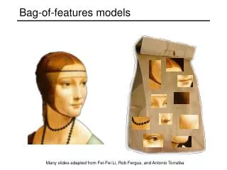
Bag-of-features for category recognition Cordelia Schmid
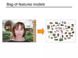
Bag-of-features for image classification • Origin: texture recognition • Texture is characterized by the repetition of basic elements or textons Julesz, 1981; Cula & Dana, 2001; Leung & Malik 2001; Mori, Belongie & Malik, 2001; Schmid 2001; Varma & Zisserman, 2002, 2003; Lazebnik, Schmid & Ponce, 2003
Texture recognition histogram Universal texton dictionary Julesz, 1981; Cula & Dana, 2001; Leung & Malik 2001; Mori, Belongie & Malik, 2001; Schmid 2001; Varma & Zisserman, 2002, 2003; Lazebnik, Schmid & Ponce, 2003
US Presidential Speeches Tag Cloudhttp://chir.ag/phernalia/preztags/ Bag-of-features for image classification • Origin: bag-of-words • Orderless document representation: frequencies of words from a dictionary • Classification to determine document categories
Bag-of-features for image classification SVM Extract regions Compute descriptors Find clusters and frequencies Compute distance matrix Classification [Nowak,Jurie&Triggs,ECCV’06], [Zhang,Marszalek,Lazebnik&Schmid,IJCV’07]
Bag-of-features for image classification SVM Extract regions Compute descriptors Find clusters and frequencies Compute distance matrix Classification Step 1 Step 3 Step 2 [Nowak,Jurie&Triggs,ECCV’06], [Zhang,Marszalek,Lazebnik&Schmid,IJCV’07]
bikes books building cars people phones trees Bag-of-features for image classification • Excellent results in the presence of background clutter
Examples for misclassified images Books- misclassified into faces, faces, buildings Buildings- misclassified into faces, trees, trees Cars- misclassified into buildings, phones, phones
Bag-of-features for image classification SVM Extract regions Compute descriptors Find clusters and frequencies Compute distance matrix Classification Step 1 Step 3 Step 2 [Nowak,Jurie&Triggs,ECCV’06], [Zhang,Marszalek,Lazebnik&Schmid,IJCV’07]
Harris-Laplace Laplacian Step 1: feature extraction • Scale-invariant image regions + SIFT • Selection of characteristic points
Step 1: feature extraction • Scale-invariant image regions + SIFT • Robust description of the extracted image regions 3D histogram image patch gradient x y • SIFT [Lowe’99] • 8 orientations of the gradient • 4x4 spatial grid
Step 1: feature extraction • Scale-invariant image regions + SIFT • Selection of characteristic points • Robust description of these characteristic points • Affine invariant regions give “too” much invariance • Rotation invariance in many cases “too” much invariance
Step 1: feature extraction • Scale-invariant image regions + SIFT • Selection of characteristic points • Robust description of these characteristic points • Affine invariant regions give “too” much invariance • Rotation invariance in many cases “too” much invariance • Dense descriptors • Improve results in the context of categories (for most categories) • Interest points do not necessarily capture “all” features
Dense features - Multi-scale dense grid: extraction of small overlapping patches at multiple scales - Computation of the SIFT descriptor for each grid cells
Step 1: feature extraction • Scale-invariant image regions + SIFT (see lecture 2) • Dense descriptors • Color-based descriptors • Shape-based descriptors
Bag-of-features for image classification SVM Extract regions Compute descriptors Find clusters and frequencies Compute distance matrix Classification Step 1 Step 3 Step 2
… Step 2: Quantization
Step 2:Quantization Clustering
Step 2: Quantization Visual vocabulary Clustering
Step 2: Quantization • Cluster descriptors • K-mean • Gaussian mixture model • Assign each visual word to a cluster • Hard or soft assignment • Build frequency histogram
K-means clustering • We want to minimize sum of squared Euclidean distances between points xi and their nearest cluster centers Algorithm: • Randomly initialize K cluster centers • Iterate until convergence: • Assign each data point to the nearest center • Recompute each cluster center as the mean of all points assigned to it
K-means clustering • Local minimum, solution dependent on initialization • Initialization important, run several times • Select best solution, min cost
From clustering to vector quantization • Clustering is a common method for learning a visual vocabulary or codebook • Unsupervised learning process • Each cluster center produced by k-means becomes a codevector • Provided the training set is sufficiently representative, the codebook will be “universal” • The codebook is used for quantizing features • A vector quantizer takes a feature vector and maps it to the index of the nearest codevector in a codebook • Codebook = visual vocabulary • Codevector = visual word
Visual vocabularies: Issues • How to choose vocabulary size? • Too small: visual words not representative of all patches • Too large: quantization artifacts, overfitting • Computational efficiency • Vocabulary trees (Nister & Stewenius, 2006) • Soft quantization: Gaussian mixture instead of k-means
Hard or soft assignment • K-means hard assignment • Assign to the closest cluster center • Count number of descriptors assigned to a center • Gaussian mixture model soft assignment • Estimate distance to all centers • Sum over number of descriptors • Frequency histogram
….. Image representation frequency codewords
Bag-of-features for image classification SVM Extract regions Compute descriptors Find clusters and frequencies Compute distance matrix Classification Step 1 Step 3 Step 2
Step 3: Classification • Learn a decision rule (classifier) assigning bag-of-features representations of images to different classes Decisionboundary Zebra Non-zebra
Classification • Assign input vector to one of two or more classes • Any decision rule divides input space into decision regions separated by decision boundaries
Nearest Neighbor Classifier • Assign label of nearest training data point to each test data point from Duda et al. Voronoi partitioning of feature space for 2-category 2-D and 3-D data Source: D. Lowe
K-Nearest Neighbors • For a new point, find the k closest points from training data • Labels of the k points “vote” to classify • Works well provided there is lots of data and the distance function is good k = 5 Source: D. Lowe
Linear classifiers • Find linear function (hyperplane) to separate positive and negative examples Which hyperplaneis best? SVM (Support vector machine)
Functions for comparing histograms • L1 distance • χ2 distance • Quadratic distance (cross-bin)
Kernels for bags of features • Histogram intersection kernel: • Generalized Gaussian kernel: • D can be Euclidean distance, χ2distance,Earth Mover’s Distance, etc.
Chi-square kernel • Multi-channel chi-square kernel • Channel c is a combination of detector, descriptor • is the chi-square distance between histograms • is the mean value of the distances between all training sample • Extension: learning of the weights, for example with MKL
Pyramid match kernel • Weighted sum of histogram intersections at multiple resolutions (linear in the number of features instead of cubic) optimal partial matching between sets of features
Pyramid Match Histogram intersection
matches at this level matches at previous level Difference in histogram intersections across levels counts number ofnew pairs matched Pyramid Match Histogram intersection
histogram pyramids number of newly matched pairs at level i measure of difficulty of a match at level i Pyramid match kernel • Weights inversely proportional to bin size • Normalize kernel values to avoid favoring large sets
Example pyramid match Level 0
Example pyramid match Level 1
Example pyramid match Level 2
Example pyramid match pyramid match optimal match
Summary: Pyramid match kernel optimal partial matching between sets of features difficulty of a match at level i number of new matches at level i
Spatial pyramid matching • Add spatial information to the bag-of-features • Perform matching in 2D image space [Lazebnik, Schmid & Ponce, CVPR 2006]
Related work • Similar approaches: • Subblock description [Szummer & Picard, 1997] • SIFT [Lowe, 1999] • GIST [Torralba et al., 2003] SIFT Gist Szummer & Picard (1997) Lowe (1999, 2004) Torralba et al. (2003)
level 0 Spatial pyramid representation Locally orderless representation at several levels of spatial resolution
level 1 Spatial pyramid representation Locally orderless representation at several levels of spatial resolution level 0
level 2 Spatial pyramid representation • Locally orderless representation at several levels of spatial resolution level 1 level 0