Download
1 / 34
340 likes | 536 Vues
Packing bag-of-features. ICCV 2009 Herv´e J´egou Matthijs Douze Cordelia Schmid INRIA. Introduction. Introduction Proposed method Experiments Conclusion. Introduction. Introduction Proposed method Experiments Conclusion. Bag-of-features. Extracting local image descriptors.

E N D
Packing bag-of-features ICCV 2009 Herv´eJ´egou MatthijsDouze CordeliaSchmid INRIA
Introduction • Introduction • Proposed method • Experiments • Conclusion
Introduction • Introduction • Proposed method • Experiments • Conclusion
Bag-of-features Extracting local image descriptors The histogram of visual word is weighted using the tf-idf weighting scheme of [12] & subsequently normalized with L2 norm Clustering of the descriptors & k-means quantizer(visual words) Roducing a frequency vector fi of length k
TF–IDF weighting • tf • 100 vocabularies in a document, ‘a’ 3 times • 0.03 (3/100) • idf • 1,000 documents have ‘a’, total number of documents 10,000,000 • 9.21 ( ln(10,000,000 / 1,000) ) • if-idf = 0.28( 0.03 * 9.21)
Binary BOF[12] • discard the information about the exact number of occurrences of a given visual word in the image. • Binary BOF vector components only indicates the presence or not of a particular visual word in the image. • A sequential coding using 1 bit per component, ⌈k/8⌉ bytes per image, the memory usage per image would be typically 10 kB per image [12] J. Sivic and A. Zisserman. Video Google: A text retrieval approach to object matching in videos. In ICCV, pages 1470–1477, 2003.
Inverted-file index(Sparsity) • Documents • T0 = "it is what it is" • T1 = "what is it" • T2 = "it is a banana" • Index • "a": {2} • "banana": {2} • "is": {0, 1, 2} • "it": {0, 1, 2} • "what": {0, 1}
Compressed inverted file • Compression can close to the vector entropy • Compared with a standard inverted file, about 4 times more images can be indexed using the same amount of memory • This may compensate the decoding cost of the decompression algorithm [16] J. Zobel and A. Moffat. Inverted files for text search engines. ACM Computing Surveys, 38(2):6, 2006.
Introduction • Introduction • Proposed method • Experiments • Conclusion
Projection of a BOF • Sparse projection matices • d: dimension of the output descriptor • k: dimension of the input BOF • For each matrix row, the number of non-zero components is , typically set nz = 8 for k = 1000, resulting in d = 125
Projection of a BOF • The other matrices are defined by random permutations. • For k = 12 and d = 3, the random permutation (11, 2, 12, 8; 9, 4, 10, 1; 7, 5, 6, 3) • Image i , m mini-BOFs • , ( )
Indexing structure • Quantization • The miniBOF is quantized by associated with matrix , , where is the number of codebook entries of the indexing structure. • The set of k-means codebooks is learned off-line using a large number of miniBOF vectors, here extracted from the Flickr1M* dataset. The dictionary size associated with the minBOFs is not related to the one associated with the initial SIFT descriptors, hence we may choose . We typically set = 20000.
Indexing structure • Binary signature generation • The miniBOF is projected using a random rotation matrix R, producing d components • Each bit of the vector is obtained by comparing the value projected by R to the median value of the elements having the same quantized index. The median values for all quantizing cells and all projection directions are learned off-line on our independent dataset
Quantizing cells [4] H. Jegou, M. Douze, and C. Schmid. Hamming embedding and weak geometric consistency for large scale image search. In ECCV, 2008.
Indexing structure • miniBOF associated with image i is represented by the tuple • total memory usage per image is bytes
Multi-probe strategy • retrieving not only the inverted list associated with the quantized index , but the set of inverted lists associated with the closest tcentroidsof the quantizer codebook • T times image hits
Fusion • Query signature • Database signature
Fusion • equal to 0 for images having no observed binary signatures • equal to if the database image i is the query image itself
Introduction • Introduction • Proposed method • Experiments • Conclusion
Dataset • Two annotated Dataset • INRIA Holidays dataset [4] • University of Ken-tucky recognition benchmark [9] • Distractor dataset • one million images downloaded from Flickr, Flickr1M • Learning parameters • Flickr1M∗
Detail • Descriptor extraction • Resize to a maximum of 786432 pixels • Performed a slight intensity normalization • SIFT • Evaluation • Recall@N • mAP • Memory • Image hits • Parameters # Using a value of nz between 8 and 12 provides the best accuracy for vocabulary sizes ranging from 1k to 20k.
mAP • Mean average precision • EX: • two images A&B • A has 4 duplicate images • B has 5 duplicate images • Retrieval rank A: 1, 2, 4, 7 • Retrieval rank B: 1, 3, 5 • Average precision A = (1/1+2/2+3/4+4/7)/4=0.83 • Average precision B = (1/1+2/3+3/5+0+0)/3=0.45 • mAP= (0.83+0.45)/2=0.64
Table 1(Holidays) # The number of bytes used per inverted list entry is 4 bytes for binary BOF & 5 bytes for BOF
Figure(Holidays+Flickr1M) # Our approach requires 160 MB for m = 8 and the query is performed in 132ms, to be compared, respectively, with 8 GB and 3s for BOF.
Introduction • Introduction • Proposed method • Experiments • Conclusion
Conclusion • This paper have introduced a way of packing BOFs:miniBOFs • An efficient indexing structure for rapid access and an expected distance criterion for the fusion of the scores • Reduces memory usage • Reduces the quantity of memory scanned (hits) • Reduces query time