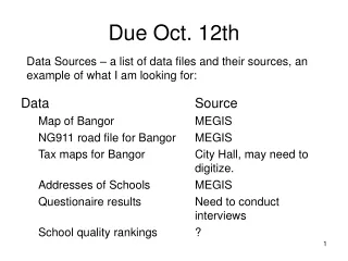
Due Oct. 12th
660 likes | 679 Vues
This project involves gathering data from various sources including a road file, tax maps, and school addresses in Bangor. The goal is to conduct interviews and create school quality rankings by October 12th.

Due Oct. 12th
E N D
Presentation Transcript
Data Source Map of Bangor MEGIS NG911 road file for Bangor MEGIS Tax maps for Bangor City Hall, may need to digitize. Addresses of Schools MEGIS Questionaire results Need to conduct interviews School quality rankings ? Due Oct. 12th Data Sources – a list of data files and their sources, an example of what I am looking for:
The .mxd File • The MXD is a template, which tells ArcMap what data to load and how to display it. • MXD not only stores maps but also stores the symbology, layout, hyperlinks, toolbars added, etc. at the time of saving the map document. Lecture 8.2
The .mxd Continued • An MXD can be distributed along with the data; hence whenever the MXD is opened the symbology, layout, order of layer always remains same. • Custom buttons or tools added to the MXD are also retained. The setting to show/hide ToolTips on toolbar can be saved in the MXD. Lecture 8.2
The .mxd Continued • MXDs can be saved to be compatible with previous versions of ArcGIS software. • But it doe NOT contain the data. Lecture 8.2
Ch. 8 Questions 1. What are the main components of a DBMS? • What are the primary functions of a DBMS? 4. What is a one-to-one relationship between tables? A many-to-one? Lecture 8.2
Which single columns in the following table may serve as keys? 9. What is the primary reason that hybrid database models are used for spatial data? Lecture 8.2
10. Does an OR condition result in more, fewer, or the same number of records than the individual component parts? 11. Does an AND condition result in more, fewer, or the same number of records than the individual component parts? Lecture 8.2
Smokers < 20% • Smokers > 20% AND illiteracy <10 • NOT (non-federal taxes > 9) • Illiteracy < 7 OR income > 22,000 • Get more federal aid than paid in taxes AND non-federal taxes > 9 • [firearm deaths < 10 AND income > 21,000] AND NOT {smokers > 20} Lecture 8.2
The GIS Database Chapter 8 – Part 2 Lecture 8.2
Reasons to Normalize a Database • There are three main reasons to normalize a database: • The first is to minimize duplicate data, • the second is to minimize or avoid data modification issues, • and the third is to simplify queries. https://www.essentialsql.com/get-ready-to-learn-sql-database-normalization-explained-in-simple-english/ Lecture 8.2
Un-normalized Data The first thing to notice is this table serves many purposes including: Identifying the organization’s salespeople Listing the sales offices and phone numbers Associating a salesperson with an sales office Showing each salesperson’s customers As a DBA this raises a red flag. In general I like to see tables that have one purpose http://www.essentialsql.com/wp-content/uploads/2014/06/Intro-Table-Not-Normalized.png Lecture 8.2
Insert Anomaly There are facts we cannot record until we know information for the entire row. In our example we cannot record a new sales office until we also know the sales person. Why? Because in order to create the record, we need provide a primary key. In our case this is the EmployeeID. Lecture 8.2
Update Anomaly The same information is recorded in multiple rows. For instance if the office number changes, then there are multiple updates that need to be made. If these updates are not successfully completed across all rows, then an inconsistency occurs. Lecture 8.2
Deletion Anomaly Deletion of a row can cause more than one set of facts to be removed. For instance, if John Hunt retires, then deleting that row cause use to lose information about the New York office. Lecture 8.2
Search and Sort Issues In the SalesStaff table if you want to search for a specific customer such as Ford, you would have to write a query like SELECT SalesOffice FROM SalesStaff WHERE Customer1 = ‘Ford’ OR Customer2 = ‘Ford’ OR Customer3 = ‘Ford’ Lecture 8.2
Normalization Rules • Begin with an unnormalized user view. • To put all tables in first normal form (1NF), remove repeating groups. • To put all tables in second normal form (2NF), remove partial dependencies. • To put all tables in third normal form (3NF) remove all transitive dependencies. Lecture 8.2
Unnormalized Table Lecture 8.2
Remove repeating groups – Creates two tables Student Table Lecture 8.2
Student_course Table Lecture 8.2
Remove partial dependencies. This refers only to tables having a composite key. You need to identify attributes that require only part of the composite key, and remove them. Registration Table
Course-Instructor Table Lecture 8.2
To put a table in third normal form remove transitive dependencies A transitive dependency is an attribute that depends only on another attribute, not a key. Course Table Lecture 8.2
Instructor Table Lecture 8.2
When NOT to Normalize • Relates in large tables require large amounts of computer time to process. • If you have an application that speed is more important than database structure. • If you are creating a very simple data base that will be used for a short time and then discarded. Lecture 8.2
Basic Spatial Analysis Ch. 9 Lecture 9
Spatial data analysis Input -> spatial operation -> output Lecture 9
Input Scope The area or extent of the input data. Local – “point” to “point” Neighborhood – adjacent regions have input Global – the entire input data layer may influence output Lecture 9
Spatial Data Analysis Usually involves manipulations or calculation of coordinates or attribute variables with a various operators (tools), such as: • Measurement • Queries & Selection • Attribute • Location • Reclassification • Dissolve • Buffering • Overlay • Clip Erase Update • Intersect Identity • Union Symmetrical Difference • Merge • Network Analysis Lecture 9
Table Operations • Statistics – count, minimum, maximum, sum, mean, standard deviation and the number of null values, as well as a frequency distribution of the variable. • Summarize - summary statistics—include the count, average, minimum, and maximum values • Join – 1:1 or m:1, two tables become one, but it is not permanent. • Relate – all other relationships, tables remain separate. • Append – Tables must have the same columns, number and type Lecture 9
Measurement: Figure 6.4 Vector GIS measurements: (a) distance and (b) area Lecture 9
Attribute Selection • A query is a question to the database. • The database response is a table. • The ArcGIS database response is selected records. If the table is the feature table it also displays the selection on the map. • Selected records can be exported to form a new shapefile/feature class. Lecture 9
Theme Name SQL Lecture 9
Spatial Selection (Select by Location) Identifying features based on spatial criteria Adjacency, connectivity, containment, arrangement Lecture 9
Adjacency depends on the algorithm used (the same is true for all spatial operations) Lecture 9
Touch the boundary of Lecture 9
Share a line segment with Lecture 9
Spatial Selection Identifying features based on spatial criteria Adjacency, connectivity, containment, arrangement Allows us to know which roads connect. Analyze transportation networks. Which river or streams flow into another. Analyze electrical networks. Lecture 9
Spatial Selection Identifying features based on spatial criteria Adjacency, connectivity, containment, arrangement Lecture 9
Selection based on spatial and non-spatial attributes Lecture 9
Spatial data analysis:Reclassification An assignment of a class or value based on the attributes or geography of an object Example: Parcels Reclassified By size Lecture 9
Spatial data analysis: Reclassification Lecture 9
Reclassify in ArcGIS Lecture 9
Natural Breaks (Jenks) • Natural Breaks classes are based on natural groupings inherent in the data. • Class breaks are identified that best group similar values and that maximize the differences between classes. • The features are divided into classes whose boundaries are set where there are relatively big differences in the data values. • Natural breaks are data-specific classifications and not useful for comparing multiple maps built from different underlying information. Lecture 9 From ArcGIS 10 Help