Lecture 10: Sampling Discrete-Time Systems

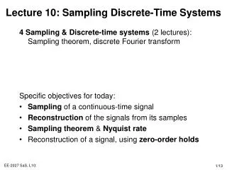
1. Lecture 10: Sampling Discrete-Time Systems • 4 Sampling & Discrete-time systems (2 lectures): Sampling theorem, discrete Fourier transform • Specific objectives for today: • Sampling of a continuous-time signal • Reconstruction of the signals from its samples • Sampling theorem & Nyquist rate • Reconstruction of a signal, using zero-order holds

2. Lecture 10: Resources • Core reading • SaS, O&W, C7 • Background reading • MIT Lectures 9 & 13 • In these two lectures, we’re going to develop the DT Fourier transform as a sampled version of the CT Fourier transform. • Note that this is opposite to time-domain convolution where we developed CT convolution as the limiting case of DT convolution

3. What is Discrete Time Sampling? • Sampling is the transformation of a continuous signal into a discrete signal • Widely applied in digital analysis systems • Sample the continuous time signal • Design and process discrete time signal • Convert back to continuous time x(t), x[n] T is the sampling period t=nT y(t) x(t) x[n] y[n] Signal reconstruction Discrete time system Discrete Time sampler

4. Why is Sampling Important? • For many systems (e.g. Matlab, …) designing and processing discrete-time systems is more efficient and more general compared to performing continuous-time system design. • How does Simulink perform continuous-time system simulation? • The signals are sampled and the systems are approximately integrated in discrete time • Mainly due to the dramatic development of digital technology resulting in inexpensive, lightweight, programmable and reproducible discrete-time systems. Widely used for communication

5. Sampling a Continuous-Time Signal • Clearly for a finite sample period T, it is not possible to represent every uncountable, infinite-dimensional continuous-time signal with a countable, infinite-dimensional discrete-time signal. • In general, an infinite number of CT signals can generate a DT signal. • However, if the signal is band (frequency) limited, and the samples are sufficiently close, it is possible to uniquely reconstruct the original CT signal from the sampled signal x1(t), x2(t), x3(t), x[n] t=nT

6. Definition of Impulse Train Sampling • We need to have a convenient way in which to represent the sampling of a CT signal at regular intervals • A common/useful way to do this is through the use of a periodic impulse train signal, p(t), multiplied by the CT signal • T is the sampling period • ws=2p/T is the sampling frequency • This is known as impulse train sampling. Note xp(t) is still a continuous time signal T

7. Analysing Impulse Train Sampling (i) • What effect does this sampling have on the frequency decomposition (Fourier transform) of the CT impulse train signal xp(t)? • By definition: • The signal p(t) is periodic and the coefficients of the Fourier Series are given by: • Therefore, the Fourier transform is given by • One property of the Fourier transform we did not consider is the multiplicative property which says if xp(t) = x(t)p(t), then

8. |X(jw)|=0: |w|>1 ws=3 Analysing Impulse Train Sampling (ii) • Substituting for P(jw) • Therefore Xp(jw) is a periodic function of w, consisting of a superposition of shifted replicas of X(jw), scaled by 1/T.

9. 1 1/T T 1 Reconstruction of the CT Signal • When the sampling frequency ws is less than twice the band-limited frequency wM, there is no overlaps the spectrum X(jw) • If this is true, the original signal x(t) can be recovered from the impulse sampled xp(t), by passing it through a low pass filter H(jw) with gain T and cutoff frequency between wM and ws-wM. wM=1 ws=3

10. Sampling Theorem • Let x(t) be a band (frequency)-limited signal • X(jw) = 0 for |w|>wM. • Then x(t) is uniquely determined by its samples {x(nT)} when the sampling frequency satisfies: • where ws=2p/T. • 2wM is known as the Nyquist rate, as it represents the largest frequency that can be reproduced with the sample time • The result makes sense because a frequency-limited signal has a limited amount of information that can be fully captured with the sampled sequence {x(nT)} X(jw) ws wM -wM w

11. x(t) t xp(t) t x0(t) t Zero Order Hold Sampling • A zero order hold is a common method for bridging CT-DT signals • A zero order hold samples the current signal and holds that value until the next sample • In most systems, it is difficult to generate and transmit narrow, large-amplitude pulses (impulse train sampling) xp(t) • We can often use a variety of filtering/interpolation techniques to reconstruct the original time-domain signal, however often the zero-order hold signal x0(t) is sufficiently accurate

12. Lecture 10: Summary • The sample time for converting a continuous time signal into a sampled, discrete time signal is determined by the Nyquist rate, amongst other things. • The signal must satisfy the relationship: • If the signal is to be preserved exactly. Information in frequencies higher than this will be lost when the signal is sampled. • A continuous time signal is often sampled and communicated using a zero order hold • Often this is enough to be considered as the re-constructed continuous time signal, but sometimes approximate methods for re-constructing the signal are used

13. Lecture 10: Exercises • Theory • SaS, O&W, 7.1-7.4, 7.7