Understanding Color Representation and Perception in Digital Systems
This text explores the fundamental aspects of color in human vision and digital systems. It covers the visible spectrum for humans and how machines perceive beyond it, introducing various coding methods like RGB, CMY, HSI, YIQ, and YUV. Additionally, it discusses the importance of color spaces in image processing, such as CIELAB, and highlights techniques like K-means clustering for color segmentation. The role of histograms in representing and matching color data is emphasized, showcasing practical applications in object recognition and classification.

Understanding Color Representation and Perception in Digital Systems
E N D
Presentation Transcript
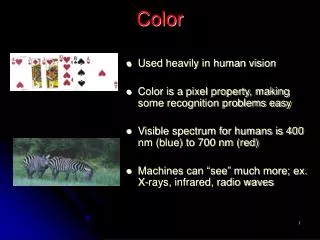
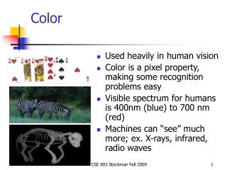
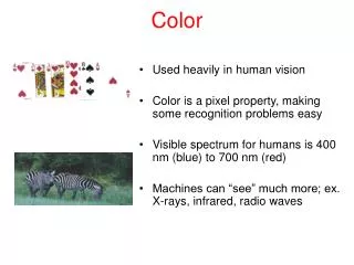
Color • Used heavily in human vision • Color is a pixel property, making some recognition problems easy • Visible spectrum for humans is 400 nm (blue) to 700 nm (red) • Machines can “see” much more; ex. X-rays, infrared, radio waves
Coding methods for humans • RGB is an additive system (add colors to black) used for displays. • CMY is a subtractive system for printing. • HSI is a good perceptual space for art, psychology, and recognition. • YIQ used for TV is good for compression.
RGB color cube • R, G, B values normalized to (0, 1) interval • human perceives gray for triples on the diagonal • “Pure colors” on corners
Color palette and normalized RGB Intensity I = (R+G+B) / 3 Normalized red r = R/(R+G+B) Normalized green g = G/(R+G+B) Normalized blue b = B/(R+G+B) Color triangle for normalized RGB coordinates is a slice through the points [1,0,0], [0,1,0], and [0,0,1] of the RGB cube. The blue axis is perpendicular to the page. In this normalized representation, b = 1 – r –g, so we only need to look at r and g to characterize the color.
Color hexagon for HSI (HSV) • Hue is encoded as an angle (0 to 2). • Saturation is the distance to the vertical axis (0 to 1). • Intensity is the height along the vertical axis (0 to 1). H=120 is green saturation intensity hue I=1 H=0 is red H=180 is cyan H=240 is blue I=0
Editing saturation of colors (Left) Image of food originating from a digital camera; (center) saturation value of each pixel decreased 20%; (right) saturation value of each pixel increased 40%.
YIQ and YUV for TV signals • Have better compression properties • Luminance Y encoded using more bits than chrominance values I and Q; humans more sensitive to Y than I,Q • Luminance used by black/white TVs • All 3 values used by color TVs • YUV encoding used in some digital video and JPEG and MPEG compression
Conversion from RGB to YIQ An approximate linear transformation from RGB to YIQ: We often use this for color to gray-tone conversion.
CIE, the color system we’ve been using in recent object recognition work • Commission Internationale de l'Eclairage - this commission determines standards for color and lighting. It developed the Norm Color system (X,Y,Z) and the Lab Color System (also called the CIELAB Color System).
CIELAB, Lab, L*a*b • One luminance channel (L) and two color channels (a and b). • In this model, the color differences which you perceive correspond to Euclidian distances in CIELab. • The a axis extends from green (-a) to red (+a) and the b axis from blue (-b) to yellow (+b). The brightness (L) increases from the bottom to the top of the three-dimensional model.
Colors can be used for image segmentation into regions • Can cluster on color values and pixel locations • Can use connected components and an approximate color criteria to find regions • Can train an algorithm to look for certain colored regions – for example, skin color
Color Clustering by K-means AlgorithmUse for HW 1 Form K-means clusters from a set of n-dimensional vectors 1. Set ic (iteration count) to 1 2. Choose randomly a set of K means m1(1), …, mK(1). 3. For each vector xi, compute D(xi,mk(ic)), k=1,…K and assign xi to the cluster Cj with nearest mean. 4. Increment ic by 1, update the means to get m1(ic),…,mK(ic). 5. Repeat steps 3 and 4 until Ck(ic) = Ck(ic+1) for all k.
K-means Clustering Example Original RGB Image Color Clusters by K-Means
Color histograms can represent an image • Histogram is fast and easy to compute. • Size can easily be normalized so that different image histograms can be compared. • Can match color histograms for database query or classification.
How to make a color histogram • Make a single 3D histogram. • Make 3 histograms and concatenate them • Create a single pseudo color between 0 and 255 by using 3 bits of R, 3 bits of G and 2 bits of B (which bits?) • Use normalized color space and 2D histograms.
Apples versus Oranges H S I Separate HSI histograms for apples (left) and oranges (right) used by IBM’s VeggieVision for recognizing produce at the grocery store checkout station (see Ch 16).
Skin color in RGB space (shown as normalized red vs normalized green) Purple region shows skin color samples from several people. Blue and yellow regions show skin in shadow or behind a beard.
Finding a face in video frame • (left) input video frame • (center) pixels classified according to RGB space • (right) largest connected component with aspect similar to a face (all work contributed by Vera Bakic)
Swain and Ballard’s Histogram Matchingfor Color Object Recognition (IJCV Vol 7, No. 1, 1991) Opponent Encoding: Histograms: 8 x 16 x 16 = 2048 bins Intersection of image histogram and model histogram: Match score is the normalized intersection: • wb = R + G + B • rg = R - G • by = 2B - R - G numbins intersection(h(I),h(M)) = min{h(I)[j],h(M)[j]} j=1 numbins match(h(I),h(M)) = intersection(h(I),h(M)) / h(M)[j] j=1
(from Swain and Ballard) 3D color histogram cereal box image
Swain and Ballard Results Results were surprisingly good. At their highest resolution (128 x 90), average match percentile (with and without occlusion) was 99.9. This translates to 29 objects matching best with their true models and 3 others matching second best with their true models. At resolution 16 X 11, they still got decent results (15 6 4) in one experiment; (23 5 3) in another.