Digital Multiplexing and Channel Banks
800 likes | 1.51k Vues
Digital Multiplexing and Channel Banks. Southern Methodist University EETS8320 Fall 2005 Lecture 6 Slides only. (No notes.). Multiplexing. Voice frequency conversations are multiplexed in traditional telephone transmission systems via

Digital Multiplexing and Channel Banks
E N D
Presentation Transcript
Digital Multiplexing and Channel Banks Southern Methodist University EETS8320 Fall 2005 Lecture 6 Slides only. (No notes.)
Multiplexing • Voice frequency conversations are multiplexed in traditional telephone transmission systems via • Frequency Division Multiplexing (FDM). - Historical system • Time Division Multiplexing (TDM), combined with digital coding of the voice signals. -Now the dominant method • Analog FDM is very similar to radio broadcasting (although via wires and not via an antenna) • FDM is used in almost all radio systems, sometimes combined with TDMA, CDMA, etc. • Only radio exception to FDMA is pulse position modulation (PPM) also called “ultra wide band,”, a recent proposal for radio purposes • Each voice signal is instantaneously modulated onto a distinct frequency sine wave for analog FDM • Typically 12 distinct modulated carrier frequencies are added and transmitted via the same wires in telephone FDM systems • Each voice signal has a pre-designated frequency receiver • FDM was the only telephone multiplexing technology used until 1961
FDM Analog Telephone Carrier • Feasible with hardware available in 1920s. • Derived from radio communication techniques • FDM reached a high state of technical refinement • Single Side Band (SSB) analog amplitude modulation (AM) (invented and analyzed by J.R. Carson) is the most spectrum-efficient method of modulation, using only about 4 kHz bandwidth per telephone voice channel • SSB still used extensively in military and amateur radio • Second and third order FDM systems hierarchy were then used to multiplex the lower order multiplex groups for more channels per link. Microwave and co-ax cable used FDM extensively in this way. • FDM installations declined after 1960s, replaced by digital multiplexing • Digital technology, although understood theoretically in 1930s, was not economically feasible until transistors and integrated circuits were developed as well
FDM Disadvantages • Basic limitations of analog amplifier noise and distortion were still present • Longer transmission distance requires more amplifiers. More amplifiers produces more audio noise and distortion • Negative Feedback design, based on the invention of H.S.Black, produces a low distortion, low noise, (high fidelity) amplifier. The noise and distortion is lower but not eliminated! • Although highly refined in design, analog hardware was still relatively costly to make, install, adjust… • With today’s integrated circuit technology, it could be improved further, (examine a cellular radio unit, for example, which uses similar analog RF technology), but would not be quite as compact and low cost as equivalent functionality using digital multiplexing
Digital Multiplexing • T-1, developed in 1961, quickly displaced FDM • An almost ideal new product: • Better speech quality than analog FDM • 24 channels; double the capacity of predecessor 12 channel analog N-carrier • Direct replacement for 2 N-carrier links • Installed cost about equal to N-carrier (thus half the cost per channel) • Cost has since reduced even further due to use of integrated circuits, etc. • Little or no field adjustment, calibration, etc. (low maintenance costs) • Most new products are not simultaneously better in price and quality, or may have backward compatibility problems
Advantages of Digital Systems and Digital TDM • The error due to digital coding and transmission in a properly functioning system can be controlled (and made very small) by the designer • The quantizing or coding error arising from encoding “round off” should be the only practical error in a properly functioning system • In a properly designed system, the difference in signal value (voltage, phase, etc..) for two distinct digital symbols is chosen to be much larger than any expected but undesired “noise” and “interference” • Practical bit error rate (BER) in a good telephone system is ~10-14 • At 50 Mb/s, one bit error occurs per 555.5 hours (23.15 days) on average • Certain processing is more feasible when the signal is represented in digital form • Digital Signal Processing (DSP), including logical processes • Encryption (where required) is simpler • Transmission of digital data and digitally coded speech should, in principle, permit less costly shared facilities (I.e., no modems needed) • This is one of the motivations for ISDN, although the promised cost savings over modem use is not fully realized with present-day ISDN
Digital Telephone Systems • Speech quality is equally good regardless of geographical distance • Delay, and thus possibly echo, is the only negative consequence of distance, and echo can be very effectively reduced to a negligible level via echo-canceling equipment • Equipment is superior to analog transmission for several reasons: • Lower initial capital and recurring (maintenance) costs • Very compact, high capacity per wire or fiber • “Cross-Fertilization” benefits from other digital technologies: • Digital switching • Computers • Data communications …all use similar technology, sometimes the exact same parts (e.g. memory, logic gates, etc.), leading to economy of scale. Design and development cost is amortized over a large quantity production.
Mild Disadvantages of Digital Systems • More complexity, more components than some cases of corresponding analog systems • Not economically feasible historically with vacuum tube hardware • Integrated circuits make this a much less significant disadvantage • A digitally coded representation of a waveform may require more bandwidth for transmission than the original analog waveform Transmission signal bandwidth is less important for wire/cable/fiber transmission than for radio transmission Use of a sophisticated encoding process can reduce this problem in some cases... For example, several low bit rate speech coders (8 kb/s or less) use less radio bandwidth for cellular and PCS radio than the corresponding analog FM radio signal, and produce similar perceived speech quality
T-1 and E-1 Use Digital Waveform Coding • Waveform coding is the first step in all types of speech coding • Waveform coding allows digital transmission of signals that must preserve the desired waveform, such as MODEM signals • Waveform coding typically produces the largest number of bits/second • More complex and sophisticated coding methods reduce the bit rate • Some waveform coding methods such as Delta modulation exploit waveform continuity • Some methods produce good encoding of the audio frequency power spectrum, but don’t preserve the waveform. OK for voice purposes.
Digital Coding of A Waveform Two Major Issues: • Required number of time samples/second • Required number and distribution of amplitude (voltage) samples We will consider these issues in that order… • How many samples per second are required to avoid missing a short-time-duration “wiggle” in the waveform? • How closely spaced must the amplitude quantizing levels be to achieve a particular accuracy goal? • One goal: hold the ratio of signal to quantizing noise below a specific level.
Telephone Voice Bandwidth Previously Standardized • Result of FDM design studies in 1920s and 1930s • 3.5 kHz upper frequency, approximately 300 Hz lower frequency. (using 3 dB “half power” points to define bandwidth) • Lowest frequency is nominally 300 Hz. • Not “high fidelity,” which requires 15 kHz to 20 kHz audio bandwidth, and low frequency response down to 20 or 30 Hz. • Inadequate to recognize some isolated phoneme sounds without benefit of known language context • Examples: f, s, sh, th (so-called fricatives) are sometimes confused • Spelling (names of alphabetic characters) b, d, t, even v etc. are sometimes confused • Requires “phonetic alphabet” for spoken spelling, like ICAO*: Alpha, Bravo, Charlie, Delta, Echo, Foxtrot,… *ICAO=International Civil Aviation Organization
Empirical Telephone Bandwidth • The nominal 3.5 kHz bandwidth for telephone voice connections was established by simple empirical testing in 1920s: • Human subjects listened to recordings of connected speech statements in their own language • Various samples were low-pass filtered with upper “cutoff” frequency adjusted • Percentage of incorrectly perceived samples was examined vs. cutoff frequency • Bandwidth which permitted ~99.9% accurate perception was used • Incidentally, narrower 2 kHz bandwidths giving only 75% accuracy were used temporarily during World War 2 to increase link capacities. • Different low frequency cutoffs (300, 500, 800 Hz) affect naturalness (“presence”) of speech, but have little effect on accuracy of understanding. • Existing telephone hardware causes ~300 Hz lower frequency cutoff, primarily from coupling transformers in subscriber loop and microphone/earphone limitations.
Why use the Narrowest Bandwidth? • Narrower signal bandwidth permits “packing” more individual channels into a fixed total bandwidth • This is particularly important in analog FDM • In digitally coded systems, less bit rate is needed to properly code a narrow band signal (more later on this point) • Engineers are usually required to build the most economical system which meets quality requirements (“Barely Adequate” system) • Systems with higher quality requirements use greater audio bandwidth: • AM Broadcasting: 5 kHz (4.5 kHz in some countries)* • FM Broadcasting: at least 15 kHz audio bandwidth • Hi-Fi audio: 20 Hz lows and 20 kHz highs (Compact Disks) * No standard on low audio frequency. Most AM broadcasts roll off at about 100 Hz.
The Nyquist* Sampling Theorem • A band-limited waveform can be accurately reconstructed if sampled at a rate greater than twice its bandwidth. • Example: a 4 kHz bandwidth signal must be sampled slightly more than 8000 samples per second • Exactly 8000 samples/sec would sample each 4000 Hz sine wave component exactly twice per cycle. • Theoretical truly band-limited signal has absolutely no audio power above some upper frequency • could be produced most practically by a test signal generator via adding several sine waves • “Real” band-limited voice signal is produced by low-pass filtering a real speech source waveform. Power above 4 kHz is 30 dB below (1/1000 of) the “in-band” typical power • Nyquist theorem does not consider amplitude quantization errors *Published by Harry Nyquist of Bell Laboratories in 1930s. Nyquist did not consider effects of digital quantization, but investigated a continuous accurate representation of each sample with perfect error-free addition of samples.
Recall: waveforms can be analyzed into sine waves Example shows one cycle (T=1 second) of a square wave and lowest three “harmonics,” sine wave components.
Fourier Analysis • How big should each sine wave component be? What is the appropriate multiplier bk for the k-th sine wave • J.B.Fourier found in 18th century that the multiplier can be found from the product integral • This formula computes the “cross correlation” coefficient between the sine wave and the square wave f(t). This is the “area” on graph paper of the product waveform from multiplying an appropriate frequency sine wave together with the waveform to be analyzed. • Because the sine wave and this particular example square wave have the same so-called “odd symmetry” we do not expect to find a cosine wave as well. In general, for non-symmetric waveforms f(t), each harmonic term comprises both a cosine and sine term.
Fourier Coefficients • From the previous formula and this particular square wave we find the first 5 coefficients: • Note that even harmonics (k=2, 4,…) are all zero. This is a special result for a “square” wave. A triangular wave has non-zero even harmonics, for example. • Incidentally, when a non-linear distortion causes peak flattening of a waveform, thus making it appear more like a square wave, we quantitatively measure this by measuring the amount of “odd harmonics” power produced due to the flattening of the peaks. This measurement is used extensively in “high fidelity” equipment descriptions.
Approx. Square Wave Using First Three Odd (1,3,5) Harmonics Proper amplitude of each “harmonic” sine wave was found from a product integral formula (same as statistical cross correlation).
Example- I • Consider a waveform like the approximate square wave made of only 3 odd-multiple frequency harmonics • The highest frequency sine wave in that example was at 5 times the basic periodic frequency • This synthetic waveform can be generated with “absolutely” no power above a specified upper frequency limit • A “filtered” real waveform has very little (but not zero) power above a specified upper frequency limit • If we can sample that highest sine wave frequently enough to capture its amplitude and phase precisely, we can reproduce it from the sample information • Sampling exactly 2 times in a cycle is not quite enough, but slightly more than 2 samples per cycle is OK • t < t/2, where t =(1/fmax) is the period of the highest frequency sine wave component. • No problem to accurately represent lower frequency sine wave components using this sampling rate
Example- II t=T/5 one cycle of 5th harmonic t/5=one cycle Two sine waves: same frequency; different amplitude, phase t=t/2 • • • • • Exactly 2 samples/cycle is ambiguous… which sine wave is it? This problem • is called “aliasing” since more than one sine wave (different amplitude and • phase) fit the same sample points.
Example- III • More than 2 samples/cycle is unambiguous. t<t/2 • • • •
Time-Domain Nyquist Rule • In the time domain, the equivalent rule is that a waveform consisting of sine waves can be measured at time intervals of t and then accurately reconstructed if the waveform has no significant “wiggles” (half-period sine wave components) which are shorter than the t time interval. • This requires examining the entire time history of the waveform, in principle. • But Fourier analysis of a waveform implies that we have examined the entire time history to compute the integral products used to evaluate the coefficients of the various sine wave terms. When we know the amplitude and phase of all the frequency components, we can “predict” the value of the sum of all frequency components for any time. • Therefore, the frequency domain statement of Nyquist’s rule implies a complete (time history) examination of the waveform’s properties. • Furthermore, telephone engineers were already used to measuring the “bandwidth” of audio signals.
Band-limited Signals • Real filtered signals cannot have zero power over a non-zero range of frequencies • OK to have zero power at discrete individual frequencies. (for example: the case of no even harmonic power for square waves) • ITU-T and other telephone systems standards call for the filter to reduce the audio power (above 4 kHz) to approximately 30 dB below (that is 1/1000 of) the mid-band power level • for example, see Bellamy (3rd Ed.): Digital Telephony, page 97, Fig. 3.6. Precise limit is 28 dB below midband audio level • This implies that “noise power” from imperfect filtration will be of a similar low magnitude • Observe that the ITU curve is ~3dB below the 0dB reference level at 3500 Hz frequency • This “3 dB or half-power point” is one of several ways to describe the bandwidth of a filter. It is easy to measure but not fully descriptive.
Digital Multiplexer Processes • Measure the voice waveform voltage to obtain 8000 samples per second • Digitally encode this voltage into a binary code value of 8 bits • Original T-1 multiplexer used a time-shared analog-digital converter • Telephone systems use a non-uniform mapping from the signal voltage to the binary code value • Serially transmit 8 bits consecutively for each such coded sample • Insert extra” bit(s) in the transmitted bit stream for synchronizing purposes • De-multiplexer operations are substantially the reverse of those listed here
Amplitude Quantization • The most obvious initial approach to amplitude quantization is to use uniform (“linear”*) voltage steps, with enough steps to quantize the largest expected amplitude into many small intervals • This is done for musical compact disk (CD) digital recording using 16 binary bits, corresponding to 65536 distinct fixed voltage levels. CD sampling rate is ~42+ ksamples/sec • Uniform quantizing is the best encoding for signals which will be processed via Digital Signal Processing (DSP) • Arithmetic adding, subtracting, etc. are straightforward • Signals not already represented by uniform quantization must be converted before DSP processing. *Yet another special jargon meaning of the word “linear”
How many bits? • 16 bits resolution is much better than is needed for telephone purposes. • Remember, the voice waveform has already been band-limited to ~3.5kHz bandwidth • Filter imperfections add about -30 dB noise (so-called “fold-over” noise) • Carbon microphone is not high-fidelity • Why bother with extra bits?? They cost more in hardware and precision of design and manufacture, and in transmission cost. • Empirical listener testing indicates about 12-13 bits of uniform resolution is adequate • No perception of degradation in telephone voice quality • Logarithmically compressed (“companded”) steps at low level permit equivalent quality with even less bits (in fact, 8)
Quantizing Noise (Round off Error) mid-tread • Whenever the actual voltage falls between two quantized amplitude steps, there is a round off error (quantization error) • The error waveform for a ramp quantized with uniform steps is shown in Bellamy (3rd Ed.), p.100, Fig.3.9. • The importance of a “mid-tread” vs. a “mid-riser” quantizer design is more significant when large quantizing steps are used. • Mid-tread has zero output unless analog input exceeds voltage step size, so background noise is suppressed, but produces worse quantizing error at low voice levels. • Mid-riser produces worse idle channel noise by increasing the miniscule background room noise or circuit noise, but has less average quantizing noise at low signal levels. • Quantizing error can be characterized as an equivalent additive quantizing “noise” Quantizer output code value Analog voltage mid-riser code value Analog voltage
Quantizing Noise • Unlike random additive noise (Gaussian noise), quantizing noise is bounded by the voltage step value of the least significant bit and has a simpler distribution of amplitude • Quantizing noise disappears during intervals of absolute silence (zero analog input) for mid-tread quantizer • For certain types of testing, artificial quantizing noise is produced by instantaneously multiplying true random noise by the instantaneous magnitude of the audio signal • The special statistical properties of quantizing noise yield a better signal-to-noise ratio than ordinary noise • 56 kb/s V.90 data modems work beyond the theoretical “Shannon limit” on their data rate because they are limited by quantizing noise, not random (Gaussian) noise
Logarithmic Companding • The human ear exhibits a phenomenon called “masking”: • a noise signal is not perceived as objectionable unless it is sufficiently large in relation to a desired sound present simultaneously • Small noises are objectionable in a quiet library • The same small noise is imperceptible at a rock concert! • This principle is the basis of noise reduction systems like the Dolby™ system for sound recording • The recording audio level is automatically increased for soft passages • The playback level is automatically reduced, to match, via an auxiliary control signal, so desired signal has the original loudness. In Dolby system, this is typically a low frequency control signal. • Therefore, noise added by the recording medium (e.g., magnetic tape “hiss”) is not noticeable during “soft” music intervals • Dolby systems treat different audio frequency bands separately (high frequency is noisiest in magnetic tape), and use different types of auxiliary signals (Dolby B, C, etc.)
Other Companding Stuff • Analog FM radio of all types (broadcast, analog cellular, specialized mobile radio -- SMR, etc.) uses time-dependent amplitude companding to reduce perceived audio background noise. • Low amplitude speech is automatically increased in power at the transmit end, reduced again at the receiver • No auxiliary time-varying control signal like Dolby’s is used, just a uniform preset adjustment which “shrinks” the amplitude scale before transmission and “stretches” the amplitude range after reception and detection of the audio • Syllabic companding in analog telephone systems (Bellamy, 3rd Ed. p.116ff) is similar • These systems have a specified time window to compute average audio power (typically 5 to 10 milliseconds)
Logarithmic Instantaneous Companding • Design objective is uniform ratio of instantaneous signal to instantaneous quantizing noise, over the range of expected amplitudes • Achieved by using approximately logarithmically spaced quantizing intervals • Quantizing error amplitude is proportional to the difference between adjacent levels, and it is then in the same proportion (call this ratio H) to the mid-level signal amplitude for each level • Power is proportional to the square of voltage amplitude, so a fixed proportionality ratio (H2) holds between instantaneous mid-quantizing-level power and quantizing noise • A small practical problem: ideal logarithm is not practical for v=0, since log(0) is negative infinity
Non-Uniform Amplitude Coding • Mu (µ) Law used in North America and Japan • In conjunction with T-1 primary rate multiplexing • “A Law” used in other parts of the world • In conjunction with E-1 primary rate multiplexing • For international digital telephone voice or modem connections, a digital code converter is provided at the Mu-law end of the international link. • Each 8-bit sample is converted based typically on a look-up table • For ISDN 64 kb/s end to end international data connections, a special parameter used in the SS7 call setup (IAM) message is used to ensure that no converter is used for that particular call to avoid modifying the binary data.
Practical Logarithmic Companding- Coding • Two methods to “shift” the logarithmic function: • µ law: Shift to left so it goes through v=0 by adding a constant to the analog voltage input • A law: Shift up by adding a constant to the code value result, then replace a small piece with a straight tangent line from the origin to a pre-designated low voltage point µ A log(1) is zero milli Practical peak voltage is ~1.55 V (corresponds to 2mW sine wave@600
CODEC Block Diagram Sample time interval: 1/8000 sec or 125 µs volts volts volts 3.5 kHz “cutoff” Digital output (serial or parallel) Pulse Code Modulation (PCM) ms Analog Multiplier Analog- Digital Converter (A or - law) CODER ms analog input may contain some power above 3.5 kHz filtered (smoothed) analog signal (Pulse Amplitude Modulation- PAM) signal Low-pass Filters 8 kHz “clock” pulse train 3.5 kHz “cutoff” Digital input (serial or parallel) Sample and Hold, or Pulse Stretcher (Boxcar) Circuit analog input Digital- Analog Converter (A or - law) DECODER volts 01011010 volts v ms ms Example: 8 serial bits in 125 µs ms
Mathematical Mu (µ)-law Graphnegative voltage graph (not shown) is odd-symmetric replica of this, but -127 code value is modified (explained later) Decimal code value Fraction of full scale 1 127 0 f(v) = ln(1+ (v/1.55))/ln(1+) where = 255 0.5 63 0 0 0 0.5 1 1.5 2 ln is natural (base e =2.718) logarithm, not decimal base. instantaneous positive voltage
Mathematical A-law Graphnegative voltage graph (not shown) is odd-symmetric replica of this Decimal code value Fraction of full scale 1 127 f(v) = (1+ ln(A(v/1.55)))/(1+ln(A)) where A= 87.6 0.5 63 observe the straight line segment starting here. Green color on color display 0 0 0 0.5 1 1.5 2 instantaneous positive voltage
T-1 (DS-1) TDM Frame 125 s or 1/8000 second F 1 2 3 4 5 6 7 8 9 10 11 12 13 14 15 16 17 18 19 20 21 22 23 24 24 8-bit PCM samples per frame, plus one framing bit per frame one time slot One framing pulse per frame bit label: 1 2 3 4 5 6 7 8 5.18 s/slot Except when common channel signaling is used (in slot 24 of one link for control of a group of links), bit 8 is “robbed” and replaced by a signaling status bit in all slots during one of 6 frames. Signaling synch is related to a 12 or 24 frame sequence established by the framing bit pattern. 8000 frames/s 193 bits/frame 1.544 Mbit/s bit rate 0.647 s/bit
E-1 (CEPT, MIC) Frame 125 s or 1/8000 second 0 1 2 3 4 5 6 7 8 9 10 11 12 13 14 15 16 17 18 19 20 21 22 23 24 25 26 27 28 29 30 31 32 8-bit time slots per frame, normally 30 used for subscriber PCM, two for synch and signals one time slot Slot zero contains synchronizing bit pattern and some trouble-shooting bit patterns. Slot 16 contains common channel signaling, either channel associated condition bits, or CCS7 bit label: 1 2 3 4 5 6 7 8 3.9 s/slot 8000 frames/s 256 bits/frame 2.048 Mbit/s bit rate 0.488 s/bit
Important Facts • Both µ-law and A-law coders use 8 bits for each sample • For international calls, a “translation” via ROM table look-up is done between A and µ (in the µ law country) • When arithmetic operations must be done (for example, for echo cancellation), the 8 bit code sample must be converted into a 12 bit (or more) sample via a look-up table or other means • 16 bits (with ~12 bit accuracy) is also used • Performing arithmetic directly on companded Mu or A values would not be meaningful • Not even a precise logarithmic value is used in the coding. The result of adding is not the sum of two logarithms exactly (although it is numerically close for large amplitude values)
Other Facts • Both µ-law and A-law use a sign and magnitude representation of the coded value • Physical zero volts has two codes: +0 and -0 • Virtually all computers today use two’s-complement coding instead to represent negative numbers • Conversion from 8-bit telephonic PCM codes to 12-bit numeric codes for DSP must correct for this as well • µ-law intentionally modifies the largest negative coded value to prevent occurrence of all-zero codes after bit inversion occurs for line coding (to be explained). A-law does not do this. • In many transmission systems using µ-law, the 8th bit is modified for signaling reasons (to be explained) in some frames of data
Practical Companding • The earliest 8-bit uniform Analog/Digital (A/D) converters used in D1 version of T-1 systems used non-linear instantaneous logarithmic companding. • Companding was achieved using an analog non-linear amplifier • Semiconductor diodes have reasonably accurate logarithmic relationship between current and voltage over part of their operating range. This was the technical basis of logarithmic companding. • In contrast, present T-1 and E-1 designs first perform ~13 bit uniform A/D conversion, then produce a companded 8-bit binary number by table lookup of an approximate µ-law (or A-law) table. (Uniform A/D conversion may use Sigma-Delta digitization.) • This table represents many straight diagonal line segments which approximate the smooth µ-law formula curve
Sign-magnitude vs. 2’s Complement Sign-magnitude still used in some CDC, Cray, Sun super-computers This value is not used in µ-law voice encoding.
Channel Banks, etc.. • The first digital telephone product was the T-1 Digital Carrier (multiplexer) • Developed at AT&T (now Lucent) Bell Labs, circa 1961 • Time Division Multiplexing (TDM) • Digital coding of speech waveforms (Mu-law companding) • Connected to analog lines and switches as required • Steadily displaced analog multiplexers • Digital switches directly using T-1 links appeared in 1970s • First AT&T ESS No.4 for transit switching • Then many digital PBX switches (Rolm, etc..) • Digital end office switches (Nortel DMS-10, DMS-100, etc.) • Today digital transmission and switching serve well over 99% of North American calls
Channel Bank • Packaging: 24 channel service units (printed wiring cards) abbreviated CSU (30 CSUs in E-1) • Common module cards • Power, line, trunk connections at back Common (shared) equipment: codecs, power supply, bit multiplexer/demux Approx. 19in (490mm) standard “rack” width
Typical T-1 Installation Channel Bank Some repeaters omitted from this figure. Channel Bank Repeater spacing 6000 ft. (1800 m) of wire. 4-wire (2 pairs) …. …. • Each channel bank supports 24 voice-grade circuits • Repeaters regenerate “clean” digital pulses with corrected timing, amplitude, pulse shape • Repeaters are powered via -130 V dc from channel bank units, using “phantom circuit” feed on both pairs. • When last wire section is too short, a “line build-out” (LBO) circuit pack is wired in to produce similar signal attenuation and related effects. • LBO consists of inductors, resistors, capacitors comprising circuit model for “missing”wire section(s). See previous transmission line lectures. • E-1 primary rate channel banks are similar, but have 30 traffic channels, 2000 m (6562 ft) repeater spacing. Repeater Repeater Repeater Maximum span ~150 miles, due to timing requirements.
Some CSU Types and Applications • 4-wire (used for various trunks or data services) • No signaling (except audio in-band tones) • Various signaling supervision options (A-B bits, E&M, etc..) • Digital data 56/64 kb/s (RS-232 or RS-449 connector) • 2-wire (various applications) • No signaling (except audio in-band tones) • Supervision for one-way or both-way trunk line: • Various types of supervision • Operates like a telephone set (connect to CO) • dc loop current on and off • responds/passes on ringing voltage • Operates like a CO switch (connect to tel set)1 • Provides loop battery, ringing • A channel with previous two CSUs at opposite ends will extend a subscriber telephone loop via a T-1 link channel. 1Requiresoptional special ringing power supply
Channel Bank Applications 4-wire • Trunk line between switches with signaling • Private tie-line between switches or similar equipment • Standard Mu-law 24 channel link • 48 channel link using ADPCM or other low bit-rate coding • Cellular link from MSC central switch to each cell • Lately, use of low bit-rate traffic channel coding (13 kb/s or less) for cellular/PCS has led to use of specialized multiplexers rather than standard channel banks. 2-wire • Non-concentrating remote • Provides “pair gain”-- 24 channels on 4 wires (with T-1 repeaters, of course) • Distinguish this from SLC-96 or similar remote concentrator which has more telephone sets than channels
Digital Symbols • Separate distinct signal voltage for each binary “bit” • BIT is a contraction of “binary digit,” a term invented by pioneer information theorist Claude Shannon • Two (voltage) levels represent the two binary symbolic values • Most popular text symbols are 1 and 0 (also T,F; or H,L) • Voltages are often 5 and 0.2 volts (TTL), or ~3 and 0.2 V in some newer portable equipment (convenient for 3 V batteries), or 12 and 0.2 V in some older equipment. • 0.2 V is often called zero. It is the natural “knee” voltage of many electronic semiconductor junction devices at their practical minimum voltage. • Design objective is two voltage levels more separated than any undesired voltages from interference, noise etc.. • In some (“active low”) designs, inverse mapping is used between symbols and voltages. Not used in this course to minimize confusion.
Parallel vs. Serial Binary • Parallel: Every bit appears on a separate wire, simultaneously • Parallel processes require more hardware, but operation is “faster” due to simultaneous activity. • Successive parallel values require simultaneous change in all bit signals. Difficult to hold parallel synchronism with many long-distance separate wire or fiber channels. • All parallel signals must be reliable for good operation. Error in one bit makes entire set of parallel bits unusable. • Parallel format used mainly within one module or cabinet of equipment for very short (< 1meter) transmission distance • Serial: Every bit appears for a preset time interval, in preset serial order, on one wire circuit. • Serial processes are slower, but use less hardware • Favored for all long distance (even a few meters) connections • Shift Register device converts between Serial and Parallel formats
Amplifier / Comparator • A “differential” amplifier with sufficiently high amplification suddenly “switches” from low to high output when two input voltages are substantially equal. vo Graphic Symbol 4 V v1 voltage amplification=2 vo v2 voltage amplification = 5000 Power supply and other details omitted. v1-v2 4 V 2 A linear region amplifier of this type is often called an “Operational Amplifier.” The high voltage output level may be 5 or 3 volts rather than 4 V shown here. Several examples here use 4 V, a convenient but not representative number.