Targetting and Assimilation: a dynamically consistent approach

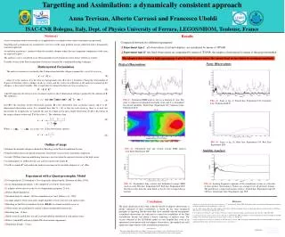
1. Targetting and Assimilation: a dynamically consistent approach Anna Trevisan, Alberto Carrassi and Francesco Uboldi ISAC-CNR Bologna, Italy, Dept. of Physics University of Ferrara, LEGOS/SHOM, Toulouse, France Summary Results • A new assimilation method and results of its application in an adaptive observations experiment are presented. • Targetting and assimiliation are considered as two faces of the same problem and are addressed with a dynamically consistent approach. • Assimilation increment is confined within the unstable subspace where the most important components of the error are expected to grow. • The analysis cycle is considered as an observationally forced dynamical system whose stability is studied. • Unstable vectors of the Data Assimilation System are estimated by a modified Breeding technique. • Mathematical Formulation • The analysis increment is confined to the N-dimensional unstable subspace spanned by a set of N vectors en: • (1) • where xa is the analysis, xf is the forecast (background) state, E is the I x N matrix (I being the total number of degrees of freedom) whose columns are the envectors and the vector of coefficients a, the analysis increment in the subspace, is the control variable . This is equivalent to estimate the forecast error covariance as: • (2) • where  represents the forecast error covariance matrix in the N-dimensional subspace spanned by the columns of E.The solution is : • (3) • here H is the (Jacobian of the) observation operator, R is the observation error covariance matrix, and yo is M-dimensional observation vector. It is intended here that N  M, so that for each vector en there is at least one observation. If, in particular, we consider the case of a single vector and a single observation, N=M=1, E consists of the single column vector e and Gof the scalar g2 . The solution is then : • (4) • Where are scalars, too. If the observation is perfect : • (5) • Outline of usage • Estimate the unstable subspace obtained by Breeding on the Data Assimilation System; • Targetted observations are placed at locations where bred vectors en have maximum component; • A wide (2500km) Gaussian modulating function is used to isolate the regional structure of the bred vector; • A small number N of Bred Vectors are used to construct the matrix E; • Use E to estimate Pfand confine the analysis increment in the unstable subspace: xa = xf+ Ea; • Experiment with a Quasi-geostrophic Model • 64-longitudinal x 32-latitudinal x 5 levels periodic channel model, (Rotunno and Bao, 1996); • Land (longitudinal grid points 1-20) completely covered by observations; • 1 adaptive observation over the Ocean (longitudinal grid points 21-64); • Perfect Model hypothesis; • Standard Analysis scheme: 3D-Var assimilation over land, (Morss et al., 1999); • A single adaptive observation and a single unstable vector eis used at each analysis time; • Breeding on the Data Assimilation System (BDAS) to estimate unstable vectors e; • Observations are assimilated in control solution and perturbed trajectories; • Breeding time: 10 days; • Bred vector discarded after use and a new perturbation introduced at each analysis time; • Perfect (labeled P) and noisy (labeled N) observations experiments; • Simulation Length: 2 years; • Comparison between two different experiments: • Experiment type I: all observations, fixed and adaptive, are assimilated by means of 3DVAR • Experiment type II: the fixed observations are assimilated by means of 3DVAR; the adaptive observations by means of the proposed method The adaptive observation in both experiments is placed at the location where the current bred vector attains its maximum amplitude Noisy Observations Perfect Observations FIG (1): Normalized RMS analysis error as a function of time. The error is expressed in potential enstrophy norm and it is normalized by natural variability. Dotted line: Experiment I-P; Continous Line: Experiment II-P FIG (4): Same as fig (1); Dotted line: Experiment I-N; Continous Line: Experiment II-N FIG (5): Same as fig (3); Blue line: Experiment I-N; Red Line: Experiment II-N FIG (2): Normalized time and vertical average RMS analysis error.From Experiment II-P Stability Analysis FIG (3): Normalized time vertical and latidudinal average RMS analysis error. Blu line: Experiment I-P; Red line: Experiment II-P. Red line results from the same fields as fig (2), but averaged also in latitude FIG (6): Leading Lyapunov exponent of the assimilation system as a function of time (perfect observations). Values are averaged over all previous instants. The growth rate is expressed in units of days-1. Dotted line: Experiment type I-P (3DVar); Continuous Line: Experiment type II-P. Conclusion The main conclusion of this work is that the benefit of adaptive observations is greatly enhanced if their assimilation is based on the same dynamical principles as targetting. Results show that a few carefully selected and properly assimilated observations are sufficient to control the instabilities of the Data Assimilation System and obtain a drastic reduction of analysis error. The success obtained in the QG-Model makes us very hopeful that, even in an operational environment with real adaptive observations, this method can yield significant improvement of the assimilation performance. References • detailed results and theoretical discussion: Carrassi A., A. Trevisan and F. Uboldi, 2004. Deterministic Data Assimilation and Targeting by Breeding on the Data Assimilation System. Submitted to J. Atmos. Sci.. • on the 3DVar scheme: Morss R., 1999. Adaptive Observations: Idealized sampling strategy for improving numerical weather prediction. PhD thesis, Massachussets of Technology, Cambridge, MA, 225 pp. • on the QG model: Rotunno R., and J. W. Bao, 1996. A case study of cyclogenesis using a model hierarchy. Mon. Wea. Rev., 124, 1051-1066 • a previous study with a small nonlinear model: Trevisan A., and F. Uboldi, 2004. Assimilation of standard and targeted observation within the unstable subspace of the observation-analysis-forecast cycle system. J. Atmos. Sci., 61, 103-113 • update of applications in progress: Uboldi F., A. Trevisan and A. Carrassi, 2004. Developing a Dynamically Based Assimilation Method for Targeted and Standard Observations. In review for Nonlinear Process in Geophysics. A.Trevisan@isac.cnr.it CONTACTS: carrassi@fe.infn.ituboldi@thor.cst.cnes.fr Acknowledgments The authors thank Rebecca Morss and Matteo Corazza for providing the code of QG-Model and 3D-Var and for getting us started with its use. We also thank Eugenia Kalnay and Zoltan Toth for their useful comments.