Errors, Uncertainties in Data Assimilation
Errors, Uncertainties in Data Assimilation. François-Xavier LE DIMET Université Joseph Fourier+INRIA Projet IDOPT, Grenoble, France. Acknowlegment. Pierre Ngnepieba ( FSU) Youssuf Hussaini ( FSU) Arthur Vidard ( ECMWF) Victor Shutyaev ( Russ. Acad. Sci.) Junqing Yang ( LMC , IDOPT).


Errors, Uncertainties in Data Assimilation
E N D
Presentation Transcript
Errors, Uncertainties in Data Assimilation François-Xavier LE DIMET Université Joseph Fourier+INRIA Projet IDOPT, Grenoble, France
Acknowlegment • Pierre Ngnepieba ( FSU) • Youssuf Hussaini ( FSU) • Arthur Vidard ( ECMWF) • Victor Shutyaev ( Russ. Acad. Sci.) • Junqing Yang ( LMC , IDOPT)
Prediction: What information is necessary ? • Model • law of conservation mass, energy • Laws of behaviour • Parametrization of physical processes • Observations in situ and/or remote • Statistics • Images
Forecast.. • Produced by the integration of the model from an initial condition • Problem : how to link together heterogeneous sources of information • Heterogeneity in : • Nature • Quality • Density
Basic Problem • U and V control variables, V being and error on the model • J cost function • U* and V* minimizes J
Optimality System • P is the adjoint variable. • Gradients are couputed by solving the adjoint model then an optimization method is performed.
Remark on statistical information • Statistical information is included in the assimilation • In the norm of the discrepancy between the solution of the model ( approximation of the inverse of the covariance matrix) • In the background term ( error covariance matrix)
Remarks: • This method is used since May 2000 for operational prediction at ECMWF and MétéoFrance, Japanese Meteorological Agency ( 2005) with huge models ( 10 millions of variable. • The Optimality System countains all the available information • The O.S. should be considered as a « Generalized Model » • Only the O.S. makes sense.
Errors • On the model • Physical approximation (e.g. parametrization of subgrid processes) • Numerical discretization • Numerical algorithms ( stopping criterions for iterative methods • On the observations • Physical measurement • Sampling • Some « pseudo-observations », from remote sensing, are obtained by solving an inverse problem.
Sensitivity of the initial condition with respect to errors on the models and on the observations. • The prediction is highly dependant on the initial condition. • Models have errors • Observations have errors. • What is the sensitivity of the initial condition to these errors ?
Optimality System : including errors on the model and on the observation
Models and Data • Is it necessary to improve a model if data are not changed ? • For a given model what is the « best » set of data? • What is the adequation between models and data?
A simple numerical experiment. • Burger’s equation with homegeneous B.C.’s • Exact solution is known • Observations are without error • Numerical solution with different discretization • The assimilation is performed between T=0 and T=1 • Then the flow is predicted at t=2.
Partial Conclusion • The error in the model is introduced through the discretization • The observations remain the same whatever be the discretization • It shows that the forecast can be downgraded if the model is upgraded. • Only the quality of the O.S. makes sense.
Remark 1 • How to improve the link between data and models? • C is the operator mapping the space of the state variable into the space of observations • We considered the liear case.
Remark 2 : ensemble prediction • To estimate the impact of uncertainies on the prediction several prediction are performed with perturbed initial conditions • But the initial condition is an artefact : there is no natural error on it . The error comes from the data throughthe data assimilation process • If the error on the data are gaussian : what about the initial condition?
Because D.A. is a non linear process then the initial condition is no longer gaussian
Remark . • The model has several sources of errors • Discretization errors may depends on the second derivative : we can identify this error in a base of the first eigenvalues of the Laplacian • The systematic error may depends be estimated using the eigenvalues of the correlation matrix
Numerical experiment • With Burger’s equation • Laplacian and covariance matrix have considered separately then jointly • The number of vectors considered in the correctin term varies
An application in oceanographyin A. Vidard’s Ph.D. • Shallow water on a square domain with a flat bottom. • An bias term is atted into the equation and controlled
RMS ot the sea surface height with or without control of the bias
An application in hydrology(Yang Junqing ) • Retrieve the evolution of a river • With transport+sedimentation
Physical phenomena • fluid and solid transport • different time scales
N 2D sedimentation modeling 1. Shallow-water equations 2. Equation of constituent concentration 3. Equation of the riverbed evolution
Semi-empirical formulas • Bed load function : • Suspended sediment transport rate : are empirical constants
An example of simulation Initial river bed • Domain : • Space step : 2 km in two directions • Time step : 120 seconds Simulated evolution of river bed (50 years)
Model error estimation controlled system • model • cost function • optimality conditions • adjoint system(to calculate the gradient)
Reduction of the size of the controlled problem • Change the space bases Suppose is a base of the phase space and is time-dependent base function on [0, T], so that then the controlled variables are changed to with controlled space size