Statistical Errors and Uncertainties: Types, Analysis, and Design Considerations
Understand different types of statistical errors (Type A and Type B), systematic errors, and poor experimental design in research. Learn how to evaluate standard uncertainties and confidence intervals using various statistical methods and models. Explore the importance of confidence intervals and probability distributions in estimating uncertainties accurately.

Statistical Errors and Uncertainties: Types, Analysis, and Design Considerations
E N D
Presentation Transcript
Random – Statistical Error From: http://socialresearchmethods.net/kb/measerr.htm
Statistical Analysis (Type A) • Type A evaluation of standard uncertainty may be based on any valid statistical method for treating data. Examples are calculating the standard deviation of the mean of a series of independent observations; using the method of least squares to fit a curve to data in order to estimate the parameters of the curve and their standard deviations; and carrying out an analysis of variance (ANOVA) in order to identify and quantify random effects in certain kinds of measurements. From: http://physics.nist.gov/cuu/Uncertainty/typea.html
Systematic Error From: http://socialresearchmethods.net/kb/measerr.htm
Systematic Analysis (Type B) • Type B evaluation of standard uncertainty is usually based on scientific judgment using all of the relevant information available, which may include: • previous measurement data, • experience with, or general knowledge of, the behavior and property of relevant materials and instruments, • manufacturer's specifications, • data provided in calibration and other reports, and • uncertainties assigned to reference data taken from handbooks. From: http://physics.nist.gov/cuu/Uncertainty/typeb.html
Poor Experimental Design! From: http://www.lhup.edu/~DSIMANEK/whoops.htm
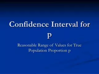
Confidence interval • Procedure: Convert an uncertainty quoted in a handbook, manufacturer's specification, calibration certificate, etc., that defines a "confidence interval" having a stated level of confidence, such as 95 % or 99 %, to a standard uncertainty by treating the quoted uncertainty as if a normal probability distribution had been used to calculate it (unless otherwise indicated) and dividing it by the appropriate factor for such a distribution. These factors are 1.960 and 2.576 for the two levels of confidence given.
Normal distribution: "99.73 %" • If the quantity in question is modeled by a normal probability distribution, there are no finite limits that will contain 100 % of its possible values. However, plus and minus 3 standard deviations about the mean of a normal distribution corresponds to 99.73 % limits. Thus, if the limits a- and a+ of a normally distributed quantity with mean (a+ + a-)/2 are considered to contain "almost all" of the possible values of the quantity, that is, approximately 99.73 % of them, then uj is approximately a/3, where a = (a+ - a-)/2 is the half-width of the interval.
Uniform (rectangular) distribution • Estimate lower and upper limits a- and a+ for the value of the input quantity in question such that the probability that the value lies in the interval a- and a+ is, for all practical purposes, 100 %. Provided that there is no contradictory information, treat the quantity as if it is equally probable for its value to lie anywhere within the interval a- to a+; that is, model it by a uniform (i.e., rectangular) probability distribution. The best estimate of the value of the quantity is then (a+ + a-)/2 with uj = a divided by the square root of 3, where a = (a+ - a-)/2 is the half-width of the interval.
Triangular distribution • The rectangular distribution is a reasonable default model in the absence of any other information. But if it is known that values of the quantity in question near the center of the limits are more likely than values close to the limits, a normal distribution or, for simplicity, a triangular distribution, may be a better model. • Estimate lower and upper limits a- and a+ for the value of the input quantity in question such that the probability that the value lies in the interval a- to a+ is, for all practical purposes, 100 %. Provided that there is no contradictory information, model the quantity by a triangular probability distribution. The best estimate of the value of the quantity is then (a+ + a-)/2 with uj = a divided by the square root of 6, where a = (a+ - a-)/2 is the half-width of the interval.
Schematic illustration of probability distributions • The following figure schematically illustrates the three distributions described above: normal, rectangular, and triangular. In the figures, µt is the expectation or mean of the distribution, and the shaded areas represent ± one standard uncertainty u about the mean. For a normal distribution, ± u encompases about 68 % of the distribution; for a uniform distribution, ± u encompasses about 58 % of the distribution; and for a triangular distribution, ± u encompasses about 65 % of the distribution.