Parameterizations in Data Assimilation
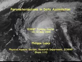
Parameterizations in Data Assimilation. ECMWF Training Course 10-12 May 2006. Philippe Lopez Physical Aspects Section, Research Department, ECMWF (Room 113). Parameterizations in Data Assimilation. Introduction Two examples of physical initialization A very simple assimilation problem

Parameterizations in Data Assimilation
E N D
Presentation Transcript
Parameterizations in Data Assimilation ECMWF Training Course 10-12 May 2006 Philippe Lopez Physical Aspects Section, Research Department, ECMWF (Room 113)
Parameterizations in Data Assimilation • Introduction • Two examples of physical initialization • A very simple assimilation problem • 3D-Var assimilation • The concept of adjoint • 4D-Var assimilation • Tangent-linear and adjoint coding • Issues related to physical parameterizations in assimilation • Physical parameterizations in ECMWF’s current 4D-Var system • Recent developments for assimilation in precipitation regions at ECMWF • Conclusions
General features of data assimilation • Goal: to produce an accurate four dimensional representation of the atmospheric state to initialize numerical weather prediction models. • This is achieved by combining in an optimal statistical way all the information on the atmosphere, available over a selected time window (usually 6 or 12 hours): • Observations with their accuracies (error statistics), • Short-range model forecast (background) with associated error statistics, • Atmospheric equilibriums (e.g. geostrophic balance), • Physical laws (e.g. perfect gas law, condensation) • The optimal atmospheric state found is called the analysis.
Which observations are assimilated? Operationally assimilated since many years ago: * Surface measurements (SYNOP, SHIPS, DRIBU,…), * Vertical soundings (TEMP, PILOT, AIREP, wind profilers,…), * Geostationarysatellites(METEOSAT, GOES,…) Polar orbiting satellites(NOAA, SSM/I, AIRS, AQUA, QuikSCAT,…): - radiances (infrared, passive microwave, visible), - products (motion vectors, total column water vapour, ozone,…). More recently: * Satellite radiances/retrievals in cloudy/precipitation regions, * Precipitation measurements from ground-based radars and gauges. Still experimental: * Satellite cloud/precipitation radar reflectivities/products, * Lidar backscattering/products (wind vectors, water vapour), * GPS water vapour retrievals, * Satellite measurements of aerosols, CO2,....
Why physical parameterizations in data assimilation? • In current operational systems, most used observations are directly or indirectly related totemperature, wind, surface pressureandhumidity outside cloudy and precipitation areas. • Physical parameterizations are used during the assimilation to link the model’s prognostic variables (typically: T, u, v, qv and Ps) to the observed quantities (e.g., radiances, reflectivities,…). • Observations related to clouds and precipitation are starting to be routinely assimilated, but how to convert such information into proper corrections of the model’s initial state (prognostic variables T, u, v, qv and, Ps) is not so obvious. For instance, problems in the assimilation can arise from the discontinuous or nonlinear nature of moist processes.
Improvements are still needed… • More observations are needed to improve the forecast of: • Mesoscale phenomena (convection, frontal regions), • Small-scale processes (planetary boundary layer and surface), • The tropical circulation (monsoons, squall lines, tropical cyclones). • Recent developments and improvements have been achieved in: • Data assimilation techniques (e.g. 3D-Var 4D-Var), • Physical parameterizations in NWP models (prognostic schemes, detailed convection and large-scale condensation processes), • Radiative transfer models (infrared and microwave frequencies), • Horizontal and vertical resolutions of NWP models (currently at ECMWF: T799 ~ 25 km, 91 vertical levels), • New satellite platforms and instruments (incl. microwave imagers, precipitation/cloud radars, lidars).
To summarize… Observations (yo) with errors a priori information from model: Background field (xb) with errors Data assimilation system (e.g., 4D-Var) Analysis (xa) • Physical parameterizations are needed: • to link the model state to the observed quantities, • to evolve the model state in time during the assimilation (e.g., 4D-Var).
Empirical Initialization • Example 1: Ducrocq et al. (2000) • Using the mesoscale research model Méso-NH (prognostic clouds and precipitation). • Particular focus on strong convective events. • Method: Prior to the forecast: • 1) A mesoscale surface analysis is performed (esp. to identify convective cold pools) • 2) the model humidity, cloud and precipitation fields are empirically adjusted to • match ground-based precipitation radar observations and METEOSAT infrared • brightness temperatures. Radar METEOSAT
12h FC from modified analysis Rain gauges + 100 km 12h FC from operational analysis + Nîmes + + Nîmes Study by Ducrocq et al. (2004) with 2.5-km resolution model Méso-NH Flash-flood over South of France (8-9 Sept 2002) Nîmes radar 12h accumulated precipitation: 8 Sept 12 UTC 9 Sept 2002 00 UTC
day-1 day 0 Newtonian relaxation time Standard Forecast Initialization with physical parameterization Example 2: Krishnamurti et al. (1988, 1993) Model state: x = (T, q, Div, Vor, Log(Ps)) Set of surface rainfall observations: Robs Kuo’s convection scheme is inverted to modify the model state so as to match the surface rainfall observations: Newtonian relaxation (or nudging) procedure over one or two days: where N is the adjustable nudging coefficient and F denotes physical and advective processes.
Physical initialization (Krishnamurti et al. 1993) 10 September 1987 1200 UTC 9 September 1987 0000 UTC 40N 30N 20N 10N Eq Satellite IR image showing hurricanes Freda, Gerald and Holly over the western Pacific. 4-day forecast of mean sea level pressure (in hPa) without (top) and with (bottom) 1-day physical initialization with SSM/I observed rainfall rates.
Important remarks on variational data assimilation • Minimizing the cost function J is equivalent to finding the so-called Best Linear Unbiased Estimator (BLUE), if: • Errors on the background and on the observations are assumed to be unbiased. • Background and observation errors are assumed to be uncorrelated. • If the statistical distributions of errors are Gaussian, then the final analysed state is also the maximum likelihood estimator of the true state. • The analysis is obtained by adding corrections to the background which depend linearly on background-observations departures. • In this linear context, the observation operator (to go from model space to observation space) must not be too non-linear in the vicinity of the model state, else the result of the analysis procedure is not optimal. • The result of the minimization depends on the background and observation error statistics (matrices B and R) but also on the Jacobian of the observation operator H.
Example of observation operator : H = convection scheme model state (T,qv) simulated surface rainfall rate Jacobians of surface rainfall rate w.r.t. T and qv Tiedtke (ECMWF’s oper mass flux) Betts-Miller (adjustment) Marécal and Mahfouf (2002)
cost function J J(xb) Jmini model variable x2 model variable x1 Finding the minimum of cost function J iterative minimization procedure
T799 L91 T255 L91 T255 L91 70 35
…3 slides of summary about 3D-Var, 4D-Var and incremental 4D-Var
3D-Var model state analysis time ta Allobservations yo between ta-3h and ta+3h are assumed to be valid at analysis time (ta=1200 UTC here) yo xa xa= final analysis xb xb= model first-guess 9 12 15 time
3 6 9 4D-Var model state analysis time ta Allobservations yo between ta-9h and ta+3h are valid at their actual time yo Model trajectory from corrected initial state xa Model trajectory from first guess xb xb Forecast model is involved in minimization 12 15 time assimilation window
Ms tangent-linear model (simplified physics) Hi tangent-linear observation operator M non-linear forecast model (full physics) H non-linear observation operator observation space Incremental 4D-Var y yoi yoj di Hixi model space H(xib) x t0 ti t0+12h time Hi trajectory from first guess x0b trajectory from corrected initial state xi Ms xib x0 x0b M t0 ti t0+12h time
y2 y1 x0 x2 x1 t1 t2 time
Summary • Variational data assimilation relies on two essential assumptions: • Gaussian distributions of model background and observation errors, • Quasi-linearity of all operators involved (H, M). • Given some background fields and a very large set of asynchronous observations available within a certain time window (e.g. 6 or 12h-long), 4D-Var searches the statistically optimal initial model state x0 that minimizes the cost function: J(x0) = Jb(x0) + Jo(HM(x0)) • The calculation of x0J requires the coding of tangent-linear and adjoint versions of the observation operator H and of the full nonlinear forecast model M (including physical parameterizations). • The tangent-linear and adjoint models M and MT are often based on a simplified version of the full nonlinear modelM to reduce computational cost in the iterative minimization and to avoid nonlinearities.
As an alternative to the matrix method, adjoint coding can be carried out using a line-by-line approach.
Basic rules for line-by-line adjoint coding (1) Adjoint statements are derived from tangent linear ones in a reversed order And do not forget to initialize local adjoint variables to zero !
Basic rules for line-by-line adjoint coding (2) To save memory, the trajectory can be recomputed just before the adjoint calculations. • The most common sources of error in adjoint coding are: • Pure coding errors, • Forgotten initialization of local adjoint variables to zero, • Mismatching trajectories in tangent linear and adjoint (even slightly), • Bad identification of trajectory updates:
machine precision reached Perturbation scaling factor
y Dy (tangent-linear) Dy (nonlinear) 0 x Dx (finite size perturbation) Issues related to the use of physical parameterizations in variational data assimilation • Variational assimilation is based on the strong assumption that the analysis is • performed in a linear framework. • Weakly nonlinear observation operators can be linearized to match this condition. • However, in the case of physical processes, strong nonlinearities can occur • sometimes in the presence of discontinuous/non-differentiable processes (e.g. • switches or thresholds in cloud water and precipitation formation).
Evolution of temperature increments (24-hour forecast) with the tangent linear model using different approaches for the exchange coefficient K in the vertical diffusion scheme. Perturbations of K included in TL Perturbations of K set to zero in TL
ECMWF’s linearized simplified physical package • Five linearized simplified physical parameterizations are currently used in ECMWF’s 4D-Var(main simplifications compared to the non-linear schemes are written in red): • Vertical diffusion: turbulent mixing in the surface and planetary boundary layers. - based on K-theory and Blackadar mixing length, - exchange coefficients = f(Richardson number) (Louis et al. 1982), -perturbations of exchange coefficients are neglected. • Gravity wave drag: subgrid-scale orographic effects (Lott and Miller 1997). - only low-level blocking part is used. • Large-scale condensation: adjustment to saturation to produce stratiform precipit. - melting of snow inside layers where T becomes > 2oC, - precipitation evaporation reduced or even set to zero. • Convection: mass flux approach (Tiedtke 1989) • - only deep convection is considered, - perturbations of mass-flux are neglected, - detrainment of cloud properties in environment is disregarded. • Radiation: TL and AD forlongwave radiation only. • - calculations in the troposphere only, • - constant emissivity formulation, - no dependence of radiation on cloud fraction.
Evaluation of the tangent-linear approximation • Time evolution of analysis increments dx0 with a T63 L31 version of the ECMWF forecast model over a 24-hour period (15 March 1999). • Nonlinear model with full physics:M(x0+dx0)-M(x0) • Tangent-linear model adiabatic (no physics):Madiab(dx0) • Tangent-linear model with physics: Mphys(dx0) • Tangent-linear approximation absolute error : • e = |M(x0+dx0)-M(x0) - M(dx0)| • If the inclusion of the physics in the tangent-linear model improves the fit to the nonlinear model, then e should be reduced. • Physical parameterizations are introduced one by one.
+ vertical diffusion + large-scale condensation + vert. diff. + gravity wave drag + convection Zonal cross-sections of changes in mean absolute errors [M(x0+dx0)-M(x0)-M(dx0)] when physical parameterizations are included (T63 L31)
Example: Use of parameterizations for the assimilation of SSM/I rainy brightness temperatures in ECMWF’s 4D-Var Until June 2005, the Special Sensor Microwave/Imager (SSM/I) brightness temperatures (TBs) were directly assimilated in ECMWF’s operational 4D-Var system only in clear-sky regions. Since June 2005, 19 and 22 GHz SSM/I TBs have also been assimilated in regions affected by precipitation and clouds using an indirect 2-step approach (Mahfouf and Marécal 2002, 2003), the so-called ‘1D+4D-Var’ method (~50,000 additional observations at each cycle). • Parameterizations of moist processes (convection, large-scale condensation and microwave radiative transfer) are key components of the assimilation of such data. • Recent developments have led to more detailed parameterizations used in tangent-linear and adjoint computations: • New simplified convection scheme (Lopez and Moreau 2005) • New simplified cloud scheme (Tompkins and Janisková 2004) • Microwave Radiative Transfer Model (Bauer 2002, Moreau 2003) • Undergoing work is aiming at replacing the indirect ‘1D-Var + 4D-Var’ method by a direct assimilation of SSM/I TBs in 4D-Var (like in clear-sky regions).

