Lecture #10 EGR 260 – Circuit Analysis

1. Lecture #10 EGR 260 – Circuit Analysis Reading Assignment: Chapter 5 in Electric Circuits, 9th Edition by Nilsson Example: Determine Vo in the circuit shown below.

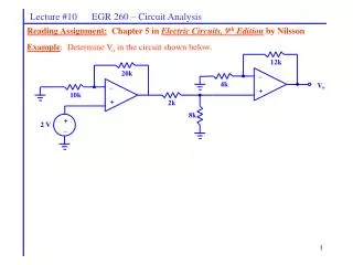
2. Lecture #10 EGR 260 – Circuit Analysis Practical Limitations in op amps Operational amplifier circuits are generally easy to analyze, design, and construct and their behavior is fairly ideal. There are, however, some limitations to op amps which the engineer should recognize. There are three primary limitations as well as some minor limitations that will be discussed in later courses. The three primary limitations in op amps are: 1) Limited voltage - In general, the output voltage is limited by the DC supply voltages. 2) Limited current - The output current has a maximum limit set by the manufacturer. 3) Frequency limitations - Op amp performance may deteriorate significantly as frequency increases (studied in later courses)

3. Lecture #10 EGR 260 – Circuit Analysis Voltage Limitations Vo for any op amp circuit is limited by the supply voltage. In general, If Vo attempts to exceed these limits, the output is limited to +VDC or -VDC and we say that the op amp is “saturated” or is “in saturation.” Practically, Vo is really about 2V under the supply voltage, or Example: Consider the inverting amplifier shown below (covered earlier). 1) Determine the voltage gain, ACL = Vo/Vin

4. Lecture #10 EGR 260 – Circuit Analysis 2) Determine Vo for various possible values of Vin (fill out the table shown below) 3) Graph Vo versus Vin . Identify the saturation and linear regions of operation. Vo Vin

5. R2 _ Vin 2k Vo + Lecture #10 EGR 260 – Circuit Analysis • Example: Consider the inverting amplifier shown below (covered earlier). • If R2 = 4k, determine range of values for Vin such that the op am will operate in the linear range • If Vin = 2V, determine R2 (max) such that the op am will operate in the linear range +12V -12V

6. 4k _ Vin 2k Vo + Lecture #10 EGR 260 – Circuit Analysis Example: Sketch Vo (on the same graph) for the circuit shown below if Vin is a triangle wave as specified below. +10V 20V -10V Vin 10V 0V -10V -20V

7. Lecture #10 EGR 260 – Circuit Analysis Current Limitations The maximum output current, Io for an op amp is specified by the manufacturer. Exceeding this limit will typically destroy the op amp. The output current can be calculated using KCL at the output node. An op amp circuit should be designed to insure that its output current does not exceed the maximum value, Io (max), specified by the manufacturer. Example: If Io (max) is specified at 25 mA by the manufacturer, determine the minimum value of RL that can safely be used in the circuit shown below.

8. Lecture #10 EGR 260 – Circuit Analysis Using node equations to analyze op amp circuits As op amp circuits become more complex, simultaneous equations may be needed to analyze them. Node equations are a natural choice since many op amp voltages are expressed as node voltages. Note: Writing a KCL (node) equation at the output node is not typically helpful except to find Io since it introduced another unknown (Io). Example: Determine Vo in the circuit shown below. Note: Writing a KCL equation (node equation) at the output is only helpful for finding Io since it introduces another unknown (Io).

9. Lecture #10 EGR 260 – Circuit Analysis Example: Determine Vo in the circuit shown below.

10. Lecture #10 EGR 260 – Circuit Analysis Example: The circuit shown below is a current amplifier. Determine an expression for IL . Also find the current gain, AI = IL/IS.

11. Lecture #10 EGR 260 – Circuit Analysis Op amp models Our analysis procedure so far has been based on making a few ideal assumptions about op amps (such as V+ = V- and I+ = I- = 0) . How would we convey these assumptions to a circuit analysis program like PSPICE? Typically, we would construct a circuit model that acts like the op amp that we desire. A simple op amp model is shown below. Also note that PSPICE can be used to model op amps with specific part numbers (such as the uA741 in the PSPICE library EVAL.SLB). In these cases, ORCAD develops very detailed circuit models that match the characteristics of the particular op amp. The ORCAD model might look like the model shown below plus additional components to more accurately model additional features. Typical values for the op amp model shown: AOL = 100,000 Rin = 2M - 10M

12. Lecture #10 EGR 260 – Circuit Analysis Example: Determine Vo in the circuit shown in two ways: 1) by making ideal op amp assumptions

13. Lecture #10 EGR 260 – Circuit Analysis Example: Determine Vo in the circuit shown in two ways: 2) by using an ideal op amp model with Rin = 2M and AOL = 100,000.

14. Lecture #10 EGR 260 – Circuit Analysis Analyzing operational amplifier circuits using PSPICE: There are two ways to analyze op amp circuits using PSPICE. 1) Use the general op amp model just introduced (consisting of a resistor and a voltage-controlled voltage source. 2) Use one of the op amp models from a library in PSPICE. Refer to two examples passed out in class (or from the instructor’s web page): 1) Op Amp Example using a General Op Amp Model 2) Op Amp Circuit using a Library Model ( uA741) Note: End of Test #2 material here.

15. Lecture #10 EGR 260 – Circuit Analysis Reading Assignment: Sections 4.9 - 4.16, in Electric Circuits, 7th Ed. by Nilsson • Network Reduction Techniques and Network Theorems • Chapter 4, Sections 9-16, in the text by Nilsson covers several useful network • reduction techniques and network theorems. • The purposes of these techniques and theorems are: • To provide alternate analysis methods • To provide methods for simplifying circuits • To provide methods for representing circuits in the simplest possible form • To gain insight into circuit behavior • Topics to be covered • Source Transformations • Superposition • Thevenin’s and Norton’s Theorems • Maximum Power Transfer Theorem

16. Lecture #10 EGR 260 – Circuit Analysis Source Transformations Before covering the actual technical of source transformations, some background on types of sources is necessary. There are two broad categories of voltage and current sources: 1) Ideal sources 2) Real sources (or practical sources) So far in the course we have only considered ideal voltage and current sources. We will now consider real sources. • Example: • The voltage supplied by an ideal 12V source will maintain 12V for any current required by the circuit. • The voltage supplied by a real 12V source (such as a car battery) will drop as the current required increases.

17. I R + S + V _ V S _ I Real Voltage Source V Lecture #10 EGR 260 – Circuit Analysis Real Voltage Source A real voltage source is modeled using an ideal voltage source, VS and a series resistance, RS. Develop an expression for I as a function of V. Plot the characteristics of a real voltage source. Also show the characteristics of an ideal voltage source.

18. Lecture #10 EGR 260 – Circuit Analysis • Example: A car battery has a voltage of 13V and a current of 0A when nothing • being powered by the battery, but the voltage drops to 9V and the current is 300A • while starting the car. • A) Draw the characteristics for the battery. • B) Determine the resistance of the battery, RS. • Draw a model of the battery.

19. Lecture #10 EGR 260 – Circuit Analysis • Example: (continued) • If two headlight were left on (Sylvania 9006ST Halogen Headlamps, rated for 55W at 12.8V), use the model to determine the current. Show the point on the graph. • If someone was “jump-starting” another car with this battery and accidentally touched the jumper cables together, determine the current through the cables (before they melted)! Show this point on the graph.

20. I + R P I V P _ I Real Current Source V Lecture #10 EGR 260 – Circuit Analysis Real Current Source A real current source is modeled using an ideal current source, IP and a parallel resistance, RP. Develop an expression for I as a function of V. Plot the characteristics of a real current source. Also show the characteristics of an ideal current source.