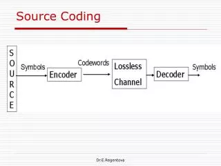
Source Coding: Part 1-Formatting

1. Source Coding: Part 1-Formatting Topics covered from Chapter 2 (Digital Communications-Bernard Sklar)Chapter 3 (Communication Systems-Simon Haykin)

3. Layering of Source Coding • Source coding includes • Formatting (input data) • Sampling • Quantization • Symbols to bits (Encoding) • Compression • Decoding includes • Decompression • Formatting (output) • Bits to symbols • Symbols to sequence of numbers • Sequence to waveform (Reconstruction)

4. Layering of Source Coding

5. Formatting • The first important step in any DCS: • Transforming the information source to a form compatible with a digital system

6. Formatting of Textual Data (Character Codes) • A textual information is a sequence of alphanumeric characters • Alphanumeric and symbolic information are encoded into digital bits using one of several standard formats, e.g, ASCII, EBCDIC

7. Character Coding (Textual Information) Example 1: • In ASCII alphabets, numbers, and symbols are encoded using a 7-bit code • A total of 27 = 128 different characters can be represented using • a 7-bit unique ASCII code

8. Formatting of Analog Data • To transform an analog waveform into a form that is compatible with a digital communication, the following steps are taken: • Sampling • Quantization and Encoding • Base-band transmission (PCM)

9. Sampling Strictly band limited Band unlimited

11. Sampling in Frequency Domain

12. Sampling Theorem • The sampling theorem for strictly band-limited signals of finite energy in two equivalent parts • Analysis : A band-limited signal of finite energy that has no frequency components higher than W hertz is completely described by specifying the values of the signal at instants of time separated by 1/2W seconds. • Synthesis : A band-limited signal of finite energy that has no frequency components higher than W hertz is completely recovered form knowledge of its samples taken at the rate of 2W samples per second. (using a low pass filter of cutoff freq. W) • Nyquist rate (fs) • The sampling rate of 2W samples per second for a signal bandwidth of W hertz • Nyquist interval (Ts) • 1/2W (measured in seconds)

13. Type of Sampling • Ideal • Natural • Practical • Sample and Hold (Flat-top)

14. Ideal Sampling ( or Impulse Sampling) x(t)x(t) x(t) Ts • Isaccomplished by the multiplication of the signal x(t) by the uniform train of impulses • Consider the instantaneous sampling of the analog signal x(t) • Train of impulse functions select sample values at regular intervals

15. Ideal Sampling

16. Practical Sampling • In practice we cannot perform ideal sampling • It is not practically possible to create a train of impulses • Thus a non-ideal approach to sampling must be used • We can approximate a train of impulses using a train of very thin rectangular pulses:

17. Natural Sampling If we multiply x(t) by a train of rectangular pulses xp(t), we obtain a gated waveform that approximates the ideal sampled waveform, known as natural sampling or gating

18. Natural Sampling • Each pulse in xp(t) has width Tsand amplitude 1/Ts • The top of each pulse follows the variation of the signal being sampled • Xs (f) is the replication of X(f) periodically every fs Hz • Xs (f) is weighted by CnFourier Series Coeffiecient • The problem with a natural sampled waveform is that the tops of the sample pulses are not flat • It is not compatible with a digital system since the amplitude of each sample has infinite number of possible values • Another technique known as flat top sampling is used to alleviate this problem; here, the pulse is held to a constant height for the whole sample period • This technique is used to realize Sample-and-Hold (S/H) operation • In S/H, input signal is continuously sampled and then the value is held for as long as it takes to for the A/D to acquire its value

19. Flat-Top Sampling Time Domain Frequency Domain

20. Flat-Top Sampling

21. Aliasing • Aliasing Phenomenon • The phenomenon of a high-frequency component in the spectrum of the signal seemingly taking on the identify of a lower frequency in the spectrum of its sampled version. • To combat the effects of aliasing in practices • Prior to sampling : a low-pass anti-alias filter is used to attenuate those high-frequency components of a message signal that are not essential to the information being conveyed by the signal • The filtered signal is sampled at a rate slightly higher than the Nyquist rate. • Physically realizable reconstruction filter • The reconstruction filter is of a low-pass kind with a passband extending from –W to W • The filter has a non-zero transition band extending form W to fstop-W • Thus use Engr. Nyquist formula Fig. a Fig. b

22. Fig. a Under-sampled Signal

23. Fig. b Over-sampled Signal

24. Pulse-Amplitude Modulation (PAM) • Output of Sampling (natural/S&H) is known as PAM • Pulse-Amplitude Modulation (PAM) • The amplitude of regularly spaced pulses are varied in proportion to the corresponding sample values of a continuous message signal. • Two operations involved in the generation of the PAM signal • Instantaneous sampling of the message signal m(t) every Ts seconds, • Lengthening the duration of each sample, so that it occupies some finite value T.

25. Other forms of Pulse Modulations

26. Other forms of Pulse Modulations • PDM (Pulse-duration modulation) • Pulse-width or Pulse-length modulation. • The samples of the message signal are used to vary the duration of the individual pulses. • PDM is wasteful of power • PPM (Pulse-position modulation) • The position of a pulse relative to its un-modulated time of occurrence is varied in accordance with the message signal.

27. Other forms of Pulse Modulations

28. Quantization

29. Average quantization noise power • Signal peak power • Signal power to average quantization noise power Out Quantized values In Quantization • Amplitude quantizing: Mapping samples of a continuous amplitude waveform to a finite set of amplitudes.

30. Quant. levels boundaries x(nTs): sampled values xq(nTs): quantized values amplitude x(t) Qunatization example 111 3.1867 110 2.2762 101 1.3657 100 0.4552 011 -0.4552 010 -1.3657 001 -2.2762 000 -3.1867 Ts: sampling time t PCM codeword 110 110 111 110 100 010 011 100 100 011 PCM sequence

32. Quantization Effect • Sampling and Quantization Effects • Quantization (Granularity) Noise: Results when quantization levels are not finely spaced apart enough to accurately approximate input signal resulting in truncation or rounding error. • Quantizer Saturation or Overload Noise: Results when input signal is larger in magnitude than highest quantization level resulting in clipping of the signal. • Timing Jitter: Error caused by a shift in the sampler position. Can be isolated with stable clock reference.

33. Non-uniform Quantization • Nonuniform quantizershave unequally spaced levels • The spacing can be chosen to optimize the Signal-to-Noise Ratio for a particular type of signal • It is characterized by: • Variable step size • Quantizer size depend on signal size

34. M any signals such as speech have a nonuniform distribution • Basic principleis to use more levels at regions with large probability density function (pdf) • Concentrate quantization levels in areas of largest pdf • Or use fine quantization (small step size) for weak signals and coarse quantization (large step size) for strong signals

36. Non-uniform Quantization Non-uniform quantization is achieved by, first passing the input signal through a “compressor”. The output of the compressor is then passed through a uniform quantizer. The combined effect of the compressor and the uniform quantizer is that of a non-uniform quantizer. At the receiver the voice signal is restored to its original form by using an expander. This complete process of Compressing and Expanding the signal before and after uniform quantization is called Companding.

37. Compressor Uniform Quantizer Expander Non-uniform Quantization (Companding)

38. Compressor Uniform Quantizer Expander Non-uniform Quantization (Companding) The 3 stages combine to give the characteristics of a Non-uniform quantizer.

39. Basically, companding introduces a nonlinearity into the signal • This maps a nonuniform distribution into something that more closely resembles a uniform distribution • A standard ADC with uniform spacing between levels can be used after the compandor (or compander) • The companding operation is inverted at the receiver • There are in fact two standard logarithm based companding techniques • US standard called µ-law companding • European standard called A-law companding

40. Nonuniform quantization using companding • Companding is a method of reducing the number of bits required in ADC while achieving an equivalent dynamic range or SQNR • In order to improve the resolution of weak signals within a converter, and hence enhance the SQNR, the weak signals need to be enlarged, or the quantization step size decreased, but only for the weak signals • But strong signals can potentially be reduced without significantly degrading the SQNR or alternatively increasing quantization step size • The compression process at the transmitter must be matched with an equivalent expansion process at the receiver

41. The signal below shows the effect of compression, where the amplitude of one of the signals is compressed • After compression, input to the quantizer will have a more uniform distribution after sampling • At the receiver, the signal is expanded by an inverse operation • The process of CO M pressing and exPANDING the signal is called companding • Companding is a technique used to reduce the number of bits required in ADC or DAC while achieving comparable SQNR

42. Input/Output Relationship of Compander • Logarithmic expression Y = log X is the most commonly used compander • Thisreduces the dynamic range of Y

43. Types of Companding -Law Companding Standard (North & South America, and Japan) where • x and y represent the input and output voltages • is a constant number determined by experiment • In the U.S., telephone lines uses companding with  = 255 • Samples 4 kHz speech waveform at 8,000 sample/sec • Encodes each sample with 8 bits, L = 256 quantizer levels • Hence data rate R = 64 kbit/sec •  = 0 corresponds to uniform quantization

44. A-Law Companding Standard (Europe, China, Russia, Asia, Africa) where • x and y represent the input and output voltages • A = 87.6 • A is a constant number determined by experiment

45. Pulse Code Modulation (PCM)

46. Pulse Code Modulation (PCM) • Pulse Code Modulation refers to a digital baseband signal that is generated directly from the quantizer and encoder output • Sometimes the term PCM is used interchangeably with quantization

47. Figure 3.13(Communication System-Simon Haykin)The basic elements of a PCM system. (Topic 3.7)

48. Pulse-Code Modulation • PCM (Pulse-Code Modulation) • A message signal is represented by a sequence of coded pulses, which is accomplished by representing the signal in discrete form in both time and amplitude • The basic operation • Transmitter : sampling, quantization, encoding • Receiver : regeneration, decoding, reconstruction • Operation in the Transmitter • Sampling • The incoming message signal is sampled with a train of rectangular pulses • The reduction of the continuously varying message signal to a limited number of discrete values per second • Nonuniform Quantization • The step size increases as the separation from the origin of the input-output amplitude characteristic is increased, the large end-step of the quantizer can take care of possible excursions of the voice signal into the large amplitude ranges that occur relatively infrequently.

49. Encoding • To translate the discrete set of sample vales to a more appropriate form of signal • A binary code • The maximum advantage over the effects of noise in a transmission medium is obtained by using a binary code, because a binary symbol withstands a relatively high level of noise. • The binary code is easy to generate and regenerate