Download
1 / 36
360 likes | 456 Vues
Explore protein-protein docking methods, ZDOCK algorithm, molecular mechanics, energy minimization, and molecular motion simulations. Learn about docking programs and molecular dynamics techniques.

E N D
C E N T E R F O R I N T E G R A T I V E B I O I N F O R M A T I C S V U Molecular Mechanics and dockingLecture 22Introduction to Bioinformatics2007
Today’s lecture • Protein interaction and docking • Zdock method • Molecular motion simulated by molecular mechanics
Docking - ZDOCK • Protein-protein docking • 3-dimensional (3D) structure of protein complex • starting from 3D structures of receptor and ligand • Rigid-body docking algorithm (ZDOCK) • pairwise shape complementarity function • all possible binding modes • using Fast Fourier Transform algorithm • Refinement algorithm (RDOCK) • Take top 2000 predicted structures from ZDOCK (RDOCK is too computer intensive to refine very many possible dockings) • three-stage energy minimization • electrostatic and desolvation energies • molecular mechanical software (CHARMM) • statistical energy method (Atomic Contact Energy) • 49 non-redundant unbound test cases: • near-native structure (<2.5Å) on top for 37% test cases • for 49% within top 4
Protein-protein docking • Finding correct surface match • Systematic search: • 2 times 3D space! • Define functions: • ‘1’ on surface • ‘r’ or ‘d’ inside • ‘0’ outside d r
Protein-protein docking • Correlation function: Ca,b,g = 1/N3SoSpSqexp[2pi(oa + pb + qg)/N] •Co,p,q
Docking Programs • ZDOCK, RDOCK • AutoDock • Bielefeld Protein Docking • DOCK • DOT • FTDock, RPScore and MultiDock • GRAMM • Hex 3.0 • ICM Protein-Protein docking (Abagyan group, currently the best) • KORDO • MolFit • MPI Protein Docking • Nussinov-Wolfson Structural Bioinformatics Group • …
Docking Programs Issues: • Rigid structures or made flexible? • Side-chains • Main-chains • Full atomic detail or simplified models? • Docking energy functions (purpose built force fields)
Molecular motions Proteins are very dynamic systems • Protein folding • Protein structure • Protein function (e.g. opening and closing of oxygen binding site in hemoglobin)
Protein motion • Principles • Simulation • MD • MC
The Ramachandran plotAllowed phi-psi angles Red areas are preferred, yellow areas are allowed, and white is avoided
Molecular mechanics techniques • Two basic techniques: • Molecular Dynamics (MD) simulations • Monte Carlo (MC) techniques
Molecular Dynamics (MD) simulation • MD simulation can be used to study protein motions. It is often used to refine experimentallydetermined protein structures. • It is generally not used to predict structure from sequence or to model the protein folding pathway. MD simulation can fold extended sequences to `global' potential energy minima for very small systems (peptides of length ten, or so, in vacuum), but it is most commonly used to simulate the dynamics of known structures. • Principle: an initial velocity is assigned to each atom, and Newton's laws are applied at the atomic level to propagate the system's motion through time • MD simulation incorporates a notion of time
K = kinetic energy V = potential energy q = coordinates p = momentum
Molecular Dynamics Knowledge of the atomic forces and masses can be used to solve the position of each atom along a series of extremely small time steps (on the order of femtoseconds = 10-15 seconds). The resulting series of snapshots of structural changes over time is called a trajectory. The use of this method to compute trajectories can be more easily seen when Newton's equation is expressed in the following form: The "leapfrog" method is a common numerical approach to calculating trajectories based on Newton's equation. This method gets its name from the way in which positions (r) and velocities (v) are calculated in an alternating sequence, `leaping' past each other in time The steps can be summarized as follows: v = dri/dt a = d2ri/d2t
Force field The potential energy of a system can be expressed as a sum of valence (or bond), crossterm, and nonbond interactions: The energy of valence interactions comprises bond stretching (Ebond), valence angle bending (Eangle), dihedral angle torsion (Etorsion), and inversion (also called out-of-plane interactions) (Einversion or Eoop) terms, which are part of nearly all forcefields for covalent systems. A Urey-Bradley term (EUB) may be used to account for interactions between atom pairs involved in 1-3 configurations (i.e., atoms bound to a common atom): Evalence = Ebond + Eangle + Etorsion + Eoop + EUB Modern (second-generation) forcefields include cross terms to account for such factors as bond or angle distortions caused by nearby atoms. Crossterms can include the following terms: stretch-stretch, stretch-bend-stretch, bend-bend, torsion-stretch, torsion-bend-bend, bend-torsion-bend, stretch-torsion-stretch. The energy of interactions between nonbonded atoms is accounted for by van der Waals (EvdW), electrostatic (ECoulomb), and (in some older forcefields) hydrogen bond (Ehbond) terms: Enonbond = EvdW + ECoulomb + Ehbond
energy distance f = a/r12 - b/r6Van der Waals forces The Lennard-Jones potential is mildly attractive as two uncharged molecules or atoms approach one another from a distance, but strongly repulsive when they approach too close. The resulting potential is shown (in pink). At equilibrium, the pair of atoms or molecules tend to go toward a separation corresponding to the minimum of the Lennard--Jones potential (a separation of 0.38 nanometers for the case shown in the Figure)
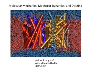
Figure: Snapshots of ubiquitin pulling with constant velocity at three different time steps.
Docking example:antibody HyHEL-63 (cyan) complexed with Hen Egg White Lysozyme (yellow) Important for binding is a salt bridge (i.e. charge complementary interaction) between Lys97 of HEL and Asp27 of the antibody heavy chain, as demonstrated by Molecular Dynamics (MD) The X-ray structure of the antibody HyHEL-63 (cyan) uncomplexed and complexed with Hen Egg White Lysozyme (yellow) has shown that there are small but significant, local conformational changes in the antibody paratope on binding. The structure also reveals that most of the charged epitope residues face the antibody. Details are in Li YL, Li HM, Smith-Gill SJ and Mariuzza RA (2000) The conformations of the X-ray structure Three-dimensional structures of the free and antigen-bound Fab from monoclonal antilysozyme antibody HyHEL-63. Biochemistry 39: 6296-6309. Salt links and electrostatic interactions provide much of the free energy of binding. Most of the charged residues face in interface in the X-ray structure. The importance of the salt link between Lys97 of HEL and Asp27 of the antibody heavy chain is revealed by molecular dynamics simulations. After 1NSec of MD simulation at 100°C the overall conformation of the complex has changed, but the salt link persists. Details are described in Sinha N and Smith-Gill SJ (2002) Electrostatics in protein binding and function. Current Protein & Peptide Science 3: 601-614.
Monte Carlo (MC) simulation • "Monte Carlo Simulation" is a term for a general class of optimization methods that use randomization. • The general idea is, given the current configuration and some figure of merit, e.g., the energy of the folded configuration, to generate a new configuration at random (or semi-random): • If the energy of the new configuration is smaller than the old configuration, always accept it as the next configuration; • if it is worse than the current configuration, accept or reject it it with some probability dependent on how much larger the new energy is than the old energy. E = E(new)-E(old) IfE<0then accept else if random[0, 1] < e-E /kTthen accept else reject Boltzmann -- probability of conformation c: P(c) = e-E(c)/kT P E
Monte Carlo (MC) simulation • The idea is that by always accepting a better configuration, on the average the system will tend to move toward a (local) energy minimum, while conversely, by sometimes accepting worse configurations, the system will be able to "climb" out of a sub-optimal local minima, and perhaps fall into the basin of attraction of the global minimum. • The specific algorithms for probabilistically generating and accepting new configurations define the type of "Monte Carlo" algorithm; some common methods are "Metropolis," "Gibbs Sampler," "Heat Bath," "Simulated Annealing," "Great Deluge," etc. • MC techniques are computationally more efficient than MD • MC simulations do not incorporate a notion of time! Local minimum Global minimum E Configuration space (models)
#! /usr/bin/perl #=============================================================================== # # $Id: mcdemo.pl,v 1.1.1.1 2003/03/12 16:13:28 jkleinj Exp $ # # mcdemo: Demo program for MC simulation of the number pi # # (C) 2003 Jens Kleinjung # # Dr Jens Kleinjung, Room P440 | jkleinj@cs.vu.nl # Bioinformatics Unit, Faculty of Sciences | Tel +31-20-444-7783 # Free University Amsterdam| Fax +31-20-444-7653 # De Boelelaan 1081A, 1081 HV Amsterdam | http://www.cs.vu.nl/~jkleinj # #=============================================================================== # preset parameters $hits = 1; $miss = 1; for ($i=0; $i<100000; $i++) { # assign random x,y coordinates $x = rand; $y = rand; # calculate radius $r = sqrt(($x*$x)+($y*$y)); # sum up hits and misses if ($r <= 1) { $hits++; } else { $miss++; } # calculate pi $pi = (4*$hits)/($hits +$miss); # print pi if ($i%100 == 0) { print("$i $pi\n"); } } #===============================================================================
In many conformational search methods based on Monte Carlo (MC), after a MC move, the system is energy minimised, i.e. put in the lowest local energy conformation, for example by gradient descent (steepest descent).
What can be done with MD and MC Dynamics of proteins • Protein folding – very difficult • Protein unfolding – done with MD • Structure refinement – most frequent application • After experimental structure elucidation • After some model building operation • PPI – Interaction dynamics, Docking • Hydrophobic patch dynamics
Take home messages • Experimentally determining protein structures • X-ray diffraction • From crystallised protein sample to electron density map • Structure descriptors: resolution, R-factor • Nuclear magnetic resonance (NMR) • Based on atomic nuclear spin • Produces set of distances between residues (distance restraints) • Distances are used to build protein model using Distance Geometry • Protein dynamics simulation • Molecular dynamics • Follows Newton’s equations of motion • Simulates molecular movements through time • Very small time steps (typically 2 femtoseconds = 2*10-15 seconds) • Protein conformational search • Monte Carlo • Conformations are randomly changed • Uses Mitropolis criterion to decide between conformation i and i+1 based on conformational internal energy and the Boltzmann equation • Has no notion of time, is a conformational search protocol • Normally faster than MD so more conformations can be generated