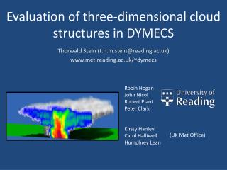
DYMECS
Thorwald Stein (t.h.m.stein@reading.ac.uk). DYMECS. Kirsty Hanley Robin Hogan John Nicol Robert Plant Thorwald Stein Emilie Carter Carol Halliwell Humphrey Lean Andrew Macallan Mal Clarke Alan Doo Darcy Ladd. The evolution of thunderstorms in the Met Office Unified Model.

DYMECS
E N D
Presentation Transcript
Thorwald Stein (t.h.m.stein@reading.ac.uk) DYMECS Kirsty Hanley Robin Hogan John Nicol Robert Plant Thorwald Stein Emilie Carter Carol Halliwell Humphrey Lean Andrew Macallan Mal Clarke Alan Doo Darcy Ladd The evolution of thunderstorms in the Met Office Unified Model
Convection-permitting models (e.g. UKV) struggle with timing and characteristics of convective storms • Model storms too regular (circular and smooth) • Not enough small storms (smaller than 40 km2) • Model storms have typical evolution (not enough variability) Nimrod UKV Original slide from Kirsty Hanley
How to evaluate thunderstorms • Track rainfall features in Nimrod data and UKV surface precipitation • Analyse bulk storm statistics (area, mean rainfall) • Use tracking information for real-time tracking with Chilbolton • Study storm height evolution • Derive vertical velocities from RHI scans through convective cores
Tracking storms • At T+1, compare image with previous time step • Use TITAN overlap method to check for storm movement: L1(T+1) K1(T) If OV(K1,L1) = A(B)/A(K1) + A(B)/A(L1) > threshold (e.g. 0.6) Then L1(T+1) is same storm as K1(T) B= (K1,L1) U
Tracking storms K4 L1 • L1 gets a new label (no overlap) • L2 gets a new label (OV(K1,L2) < threshold) • L3 gets label of K1 (OV(K1,L3) > OV(K1,L4)) and defined as “parent” • L4 gets a new label, but defined as “child” • L5 gets label of K2 (OV(K2,L5) > OV(K3,L5)) and property “accreted K2, K3” L2 K1 L3 L4 K2 L5 K3
Tracking storms K4 L1 • What if K4 were fast-moving? • Use velocity information… • Taking velocity as displacement of centroid brings trouble for breaking/merging events. • Use FFT method to track displacement between rainfall images at larger scale L2 K1 L3 L4 K2 L5 K3
Storm statistics – 07-20 UTC Too few small storms (less than 40 km2) Too few weakly precipitating storms Maximum rain-rate Storm area Too low maximum rain rate? Hail? Errors in Nimrod? Original slide from Kirsty Hanley
Storm statistics – 04-20 UTC • Bin storms by area – 10 storms per bin • Compare bin-averaged storm area with area-averaged rain-rate of each bin. Nimrod UKV Small but intense storms Small storms with weak precip Original slide from Kirsty Hanley
Sensitivity studies – total precipitation 3D Smagorinsky Prognostic graupel KK autoconversion Rhcrit = 0.99 Original slide from Kirsty Hanley
Obtain mean evolution of area Observations (Nimrod) Model (UKV 3Z) Normalised area Normalised time Normalised time … and mean rainfall
Combine area and rainfallfor mean storm life cycle Observations (Nimrod) Model (UKV 3Z) Normalised area Normalised area Normalised mean rainfall Normalised mean rainfall Modelled storms all have peak rainfall at the same time Modelled storms stay too long at peak area
Tracking storms … with Chilbolton
Prioritizing Storms 200 • Per storm, store: • Area • Azimuth • Range • [u,v] • Centroid • Bounding box • Et cetera... • Local rainfall maxima within storm (core, cell)for vertical profiles 150 100 50
Prioritizing Storms Sweet spot for RHI scans Too near: Miss tops of storm ortakes too long to finish RHI Reflectivity Height Radial winds Height Distance from radar Rainfall Too far: Miss low-level precipitationand coarser resolution
Prioritizing Storms 200 • Scan scheduler: • Read nimrod scene • Prioritize storms • Issue radar commands • Scan strategy: • 4 RHI scans through each core in (clockwise-most) storm 1 • PPI volume scan (10 PPIs) through storm 1 • Repeat for next storm (anti-clockwise) • Finish with low-level PPI back to 1 150 100 50
Tracking storm “1504” Storm tracked in Nimrod data over 3-hour period shows growth of surface rainfall area as well as intensification in mean rainfall. Mean rainfall Area
Tracking storm “1504” Height Analysis of Chilbolton volume scans shows increase in height as area remains constant. Occurrence of 40dBZ coincides with higher mean rainfall in Nimrod data. Mean rainfall Area
Tracking storm “1504” Height Analysis of Chilbolton volume scans shows increase in height as area remains constant. Occurrence of 40dBZ coincides with higher mean rainfall in Nimrod data.
Tracking storm “1504” Height Analysis of Chilbolton volume scans shows increase in height as area remains constant. Occurrence of 40dBZ coincides with higher mean rainfall in Nimrod data.
Tracking storm “1504” Storm properties can be linked to different stages in life cycle. Attempt similar approach in hourly model cloud fields by forward modelling reflectivities. UM Storm for same case Growth Stable Intensification Area
20 dBZ height statistics UKV (model) Chilbolton (obs) Morning Afternoon
Vertical velocities Red towards radar Blue away from radar Original slide from Robin Hogan
Estimation of vertical velocities from continuity Vertical cross-sections (RHIs) are typically made at low elevations (e.g. < 10°) Radial velocities provide accurate estimate of the horizontal winds Assume vertical winds are zero at the surface Working upwards, changes in horizontal winds at a given level increment the vertical wind up to that point Must account for density change with height Original slide from John Nicol
Reflectivity (dBZ) Radial velocity (m/s) Sets of four vertical scans through a convective core can be used to track radial velocity features to retrieve vertical velocities. Horizontal velocity (m/s) Vertical velocity (m/s) 10:55 UTC26/08/2011 2D wind field (m/s) Original slide from John Nicol
Strong convection w ≈1.7m/s 07/08 26/08 27/08 03/11 Moderate convection w ≈1.3m/s 04/11 13/12 Simple categorisation by std. dev. of vertical velocities (dBZ>15) Moderate convection w ≈0.9m/s 14/12 26/01 03/03 10/04 11/04 Weak convection w ≈0.5m/s 23/08 07/03 04/04 Original slide from John Nicol
Assumptions Assume that convergence at the lowest detectable level extends down to the surface No divergence into plane from cross-radial winds Likely to be true for linear structures (e.g. fronts) orientated perpendicular to the radar scan but not for circular structures. Vertical cross-section viewed from above Radar Are vertical velocities underestimated in cases such as this? By a factor two? Original slide from John Nicol
Discussion • Small storms: Need to go to higher resolution? • Detecting convergence in dopplerized network