Generalised Predictive Control (Tuning & Implementation)
Generalised Predictive Control (Tuning & Implementation). Amir Reza Neshasteriz Peyman Bagheri. Generalized Predictive Control (Tuning & Implementation). Overview of the Presentation. GPC Formulation Proposed GPC Method (Camacho & Bordons) Extended GPC Method Pole Placement Tuning

Generalised Predictive Control (Tuning & Implementation)
E N D
Presentation Transcript
Generalised Predictive Control(Tuning & Implementation) Amir Reza Neshasteriz Peyman Bagheri
Generalized Predictive Control(Tuning & Implementation) Overview of the Presentation • GPC Formulation • Proposed GPC Method (Camacho & Bordons) • Extended GPC Method • Pole Placement Tuning • Tuning Based on Analysis of Variance (ANOVA) • GPC application in a PH plant • Implementation of GPC
Introduction to Generalised Predictive Controllers • CARIMA Model : • Cost Function : • Control Signal :
Introduction to Generalised Predictive Controllers • Exercising Receding Horizon Concept : • Applying the input to the system • Calculating Output with respect to the reference
Proposed GPC methodBy Camacho & Bordons First Order System Estimation : CARIMA Prediction : Calculating Input Sequence :
Proposed GPC methodBy Camacho & Bordons Considering and Receding Horizon Concept : Controller Coefficients :
Advantages& Limitations Advantages and Improvements Compared to conventional method: Less Computational Burden Ability and capacity for utilization in most process applications Simplicity regarding implementation Limitations : Application restricted to First order estimates (Oscillating Modes Neglected) Effects of presumable zeros excluded Choosing lambda heuristically Lack of tuning Solution Second/Higher Order Estimation+Tuning
Extended GPC methodSecond Order Systems • Second Order System Estimation : • CARIMA Prediction : • Calculating Input Sequence :
Controller Coefficients General Predictor (Equivalent Structure) : Converting to Vector-Matrix format : Minimizing Cost Function with respect to Input Sequence :
Controller Coefficients Calculating Input (Receding Horizon) : Controller Surfaces are constructed using the following assumptions :
Calculating Coefficients Surfaces Estimates As it can be seen in previous plots for the two poles, changes in coefficients are symmetric. Nonlinear Regression of the surfaces yields: Iterating for ,the curves for pertaining coefficients are found using MATLAB structure programming Estimations for resultant curves are done using Nonlinear Least squares (Levenberg-Marquardt algorithm)
Table of sub-coefficients Sub-Coefficient Estimation (Second Order)
Pole Placement Tuning The object of tuning is to find a certain weighting factor λ so that certain criterions, such as performance or stability are met with:
Simulation Example (A central Heating Configuration of a building) Comparison between two tuning methods, dotted lines show tuning with and solid line shows proposed tuning method results.
Tuning Based on Analysis of Variance (ANOVA) In multi-way ANOVA it is determined whether means in a set of data differ when grouped by multiple factors. If so, it can be verified which factors or combinations of factors are associated with the difference. In other words, the effects of multiple factors on the mean of data are measured. To utilize ANOVA for our objective, some experiments have to be performed that involve SOPDT model parameters and tuning factor . It should be noted that the tuning procedure is not limited to finding an expression , and for any other parameters in GPC (such as horizons or sampling time) could be repeated.
Experiment Setup In each of these cases 256 SOPDT models are generated according to the tables. In every simulation a tuning parameter that minimizes the following cost function is acquired Subsequent to the construction of the bank of models, an analysis of variance is performed on the optimal tuning parameter as a response vector and model parameters as variables. Therefore, model parameters that have more influence on the optimal tuning parameter set could be singled out using ANOVA.
ANOVA Results From the information available from two simulations and their analysis of variance results, optimal λ set will depend on mentioned model parameters in each simulation and hence it is a function of them. To find this function, nonlinear regression has to be performed on the and model parameters. After many attempts, the following expression was derived for the real pole case with very good fit For the complex conjugate case, the expression is
Illustrative Examples Case Study 2 simulation (the gas fire burner), solid line: proposed tuning method, Dotted line: Trial and Error Method Case Study 1 simulation solid line: proposed tuning method, Dotted line: conventional method
مقدمه • مسالهرگولهسازی و کنترل فرآیند pH • غیرخطی گری شدید، نامعینی مدل و تاخیر زیاد • مدل سازی و کنترل تک ورودی- تک خروجی سیستم pH • مدل سازی و کنترل چندمتغیرهسیستم pH • بهبود عملکرد سیستم کنترل pHبه وسیله راهکارهای چندمتغیره • کنترل پیش بین تعمیم یافته • نتایج عملی پیاده سازی GPCروی سیستم pH
pH یک معیار اندازهگیری برای مقدار غلظت یون هیدرونیوم در محلول آبی است. فرآیند pH • دو دسته بندی کلی برای فرآیند pH : • بسته (batch): محلول درون مخزن بسته قرار دارد. • پیوسته: هدف کنترل pHجریان خروجی است.
مدل سازی دینامیکی فرآیند pH انواع فرآیندهای pHبر اساس تعداد ورودی و خروجیها 1. دیدگاه تک ورودی- تک خروجی 2. دیدگاه دو ورودی- دو خروجی
مدل سازی دینامیکی فرآیند pH مدل دینامیکی تک ورودی- تک خروجی منحنی تتراسیون اسید قوی باز قوی اسید ضعیف باز قوی
مدل سازی دینامیکی فرآیند pH مدل دینامیکی دو ورودی- دو خروجی
غیرخطیگری شدید سیستم pH تغییر بهره dcسیستم با تغییر نقطه کار
روشهای کنترلی برای حالت تک ورودی- تک خروجی برای حالت SISOمقالات فراوانی داده شده است، روشهایی که بیشتر مورد استفاده قرار گرفته: • کنترل پیش بین مدل چندگانه • کنترل پیش بین تعمیم یافته مدل چندگانه • کنترل تطبیقی مدل چندگانه • کنترل فازی پیش بین مدل • کنترل تطبیقی عصبی • کنترل مقاوم • الگوریتم ژنتیک • و ...
روشهای کنترلی برای حالت تک ورودی- تک خروجی تداخل نقص کنترل SISO: • حلقه کنترلی روی کانال pHبسته میشود. • در عمل نیاز داریم حجم مخزن ثابت بماند. کاری که در آزمایشگاه انجام میشود: کنترل سطح محلول با فیدبک داخلی توسط آب تغییر pHدر اثر افزودن آب
روشهای کنترلی فرآیند چندمتغیره pH ساختار کنترلر برای سیستم خطی چندمتغیره: • ساختارهای دکوپله ساز و کنترلرهای SISO • ساختار کنترلی چندمتغیره کنترل پیش بین کنترلرهای هوشمند و ... کنترل پیش بین تعمیم یافته (GPC) کنترل پیش بین مدل (MPC) 33
کنترل پیش بین تعمیم یافته (GPC) • GPC • قابل استفاده برای سیستمهای SISOو MIMOبدون پیچیدگی زیاد • امکان بکارگیری constrains • قابل استفاده برای سیستمهای تاخیردار • مقاوم بودن روش کنترلی نسبت به تغییر پارامترها
کنترل پیش بین تعمیم یافته (GPC) فرموله بندی GPCدر فضای حالت MIMO state space model: x(k+1) = A x(k) + B u(k) y(k) = C x(k) + D u(k) + dist Note: Assumes D=0 J = sum (r-y)^2 + (u(k+i-1)-uss) R (u(k+i-1)-uss) umin < ufut < umax Dumin < Dufut < Dumax