IMF Prediction with Cosmic Rays

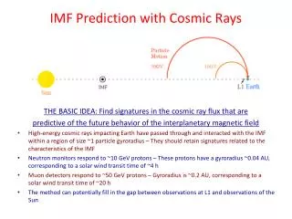
1. IMF Prediction with Cosmic Rays THE BASIC IDEA: Find signatures in the cosmic ray flux that are predictive of the future behavior of the interplanetary magnetic field • High-energy cosmic rays impacting Earth have passed through and interacted with the IMF within a region of size ~1 particle gyroradius – They should retain signatures related to the characteristics of the IMF • Neutron monitors respond to ~10 GeV protons – These protons have a gyroradius ~0.04 AU, corresponding to a solar wind transit time of ~4 h • Muon detectors respond to ~50 GeV protons – Gyroradius is ~0.2 AU, corresponding to a solar wind transit time of ~20 h • The method can potentially fill in the gap between observations at L1 and observations of the Sun

2. IMF PREDICTION WITH COSMIC RAYSBased on Quasilinear Theory (QLT)

3. ENSEMBLE-AVERAGING DERIVATION OF THE BOLTZMANN EQUATION:START WITH THE VLASOV EQUATION The equation is relativistically correct

4. ENSEMBLE AVERAGETHE VLASOV EQUATION

5. SIMPLIFY THE ENSEMBLE-AVERAGED EQUATION WITH A TRICK For gyrotropic distributions, only ψ1 matters!

6. SUBTRACT THE ENSEMBLE-AVERAGED EQUATION FROM THE ORIGINAL EQUATION… THEN LINEARIZE Why “Quasi”–Linear? 2nd order terms are retained in the ensemble-averaged equation, but dropped in the equation for the fluctuations δf

7. AFTER LINEARIZING, IT’S EASY TO SOLVE FOR δf BY THE METHOD OF CHARACTERISTICS “z” here is the mean Field direction, NOT GSE North In effect, this integrates the fluctuating force backwards along the particle trajectory. This is like tomography, but using a helical “line of sight”

8. Equations from Pei

9. Equations from Pei

10. Equations from Pei So, the integration of t is solved as

11. Spaceship Earth Spaceship Earth is a network of neutron monitors strategically deployed to provide precise, real-time, 3-dimensional measurements of the cosmic ray angular distribution: 11 Neutron Monitors on 4 continents Multi-national participation: Bartol Research Institute, University of Delaware (U.S.A.) IZMIRAN (Russia) Polar Geophysical Inst. (Russia) Inst. Solar-Terrestrial Physics (Russia) Inst. Cosmophysical Research and Aeronomy (Russia) Inst. Cosmophysical Research and Radio Wave Propagation (Russia) Australian Antarctic Dvivision Aurora College (Canada)

12. Data Pre-processing To select the intensity variation that would be sensitive to the IMF, we subtract isotropic component and 12 hour trailing-averaged anisotropy from observed NM intensity where f0and ξ are determined for each hour from the following best fit function

13. Data Pre-processing Observed intensity After subtract isotropic component And after subtract 1st order anisotropic component Data during GLE is removed

14. Best-fit to the data C = A/|A|= +1 or -1, is the magic number calculated from the amplitude of pitch angle distribution of NM data. fit this function to the cosmic ray flux and get 4 parameters Ax, Ay, px, py

15. estimation of dB * dBexp is calculated from the model in IMF coordinate as The IMF at time later is estimated from the IMF at the point Vsw*upstream from Earth, where Vsw is observed solar wind velocity. * dBobs is calculated as the deviation from 12-hour tr-moving average of observed IMF in GSE coordinate.

16. Conversion of coordinate IMF coordinate Ximf is in Xgse-Ygse plane Yimf is pointing north ward, and in Zimf-Zgse plane Zgse Yimf Zimf  = GSE longitude of IMF + 90o = GSE colatitude of IMF IMF Ximf Ygse IMF to GSE : rot + on Ximf and rot + on Zgseand  Xgse GSE to IMF : rot - on Zgseand rot - on Ximf

17. Pitch angle and Gyro Phase of the particle A : asymptotic viewing direction of particle calculated from particle trajectory code in gse coordinate then converted to imf coordinate Yimf A IMF Zimf Ximf

18. Pitch angle Gyro Phase Away GSE Lat -180 GSE Lat +180 Toward

19. ICME Events ICME Shock • Use ICME List from Richardson & Cane 2010, Solar Phys http://www.ssg.sr.unh.edu/mag/ace/ACElists/ICMEtable.html • 161 ICMEs are listed from 2001 to 2006 • Compare the IMF during the time from the IP Shock arrival time to the ICME end time • Use hourly OMNI data (time corrected ACE or WIND) for the comparison of in-situ IMF data

20. ICME Shock Estimated IMF component Observed IMF to be compared • /12

24. dt=0 dt=1 dt=2 with dt

25. Question: why we have good correlation when we use the factor C

26. 0h prediction

31. Update Feb 18 • Don’t use the future IMF data for the estimation of future IMF

32. estimation of dB * dBexp is calculated from the model in IMF coordinate as IMF xgse Vsw·Δt The IMF at time later is estimated from the IMF at the point Vsw* upstream from Earth, where Vsw is observed solar wind velocity. * dBobs is calculated as the deviation from 12-hour tr-moving average of observed IMF in GSE coordinate. Background IMF

33. ICME Shock Estimated IMF component Observed IMF to be compared • /12 : current time

36. B0=5nT

37. Update Mar 11 Estimated IMF component Observed IMF to be compared • /12 : current time

39. 0 hour predict 3 hour predict

41. 0 hour predict 3 hour predict

42. N+/Nall Mean of corr. coeff Median of corr. coeff

43. 6 years of data 0 hour prediction 5 hour prediction

44. 6 years of data (event period only) 0 hour prediction 5 hour prediction

45. 6 years of data (without event period) 0 hour prediction 5 hour prediction