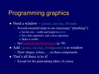
Graphics Programming

1. Graphics Programming Chun-Yuan Lin CG

2. The approach in this book for computer graphics is programming oriented. • We introduce a minimal application programmer’s interface (API) to allow you to program many interesting two- and three-dimensional problems and to familiarize you with the basic graphics concepts. • We regard two-dimensional graphics as a special case of three-dimensional graphics. The program code for two-dimensional graphics will execute without modification on a three-dimensional system. CG

3. Our development uses a simple but information problem: the Sierpinski gasket. It shows how we can generate an interesting and, to many people, unexpectedly sophisticated image using only a handful of graphics functions. • We use OpenGL, but the discussion of the underlying concepts is broad enough to encompass most modern systems. CG

4. The Sierpinski Gasket (1) • We use a sample problem the drawing of the Sierpinski gasket-an interesting shape that has a long history and is of interest in area as fractal geometry. • The sierpinski gasket is an object that can be defined recursively and randomly. • Suppose that we start with three points in space. As long as the points are not collinear, they are the vertices of a unique triangle and also define a unique plane. (we assume that z = 0, three vertices are (x1, y1, 0), (x2, y2, 0), (x3, y3, 0)) CG

5. The Sierpinski Gasket (2) • The construction proceeds as follows. Thus each time that we generate a new point, we display it on the output device. • The possible form for the graphics program might be this: main() { initialize_the_system(); for(some_number_of_points) { pt = generate_a_point(); display_the_point (pt); } Cleanup(); } CG

6. The Sierpinski Gasket (3) • First, we concentrate on the core: generating and displaying points. • We must answer two questions: • how do we represent points in space? • Should we use a two-dimensional, three-dimensional, or other representation? CG

7. Programming two-dimensional applications (1) • The larger three-dimensional world hold for the simpler two-dimensional world. • We can generate a point in the plane z = 0 as p= (x, y, 0) in the three-dimensional world, or as p = (x, y) in the two-dimensional plane. • OpenGL allows us to use either representation. We can implement representation of points in a number of ways. p= (x, y, z) or a column matrix CG

8. Programming two-dimensional applications (2) • We use the terms vertex and point in a somewhat different manner in OpenGL. A vertex is a position in space; we use two-, three-, and four-dimensional space in computer graphics. • The simplest geometric primitives is a point in space, which is specified by a single vertex. • Two vertices define a line segment. (a second primitive object) • Three vertices can determine either a triangle or a circle. • Four vertices determine a quadrilateral, and so on. • OpenGL has multiple forms for many functions. CG

9. Programming two-dimensional applications (3) • For the vertex functions, we can write the general form glVertex*() where the * can be interpreted as either two or three characters of the form nt or ntv, where n signifies the number of dimensions (2,3 or 4); t denotes the data type, such as integer (i), float (f), or double (d); and v, if present, indices that the variables are specified through a pointer to an array, rather than through an argument list. • In OpenGL, we often use basic OpenGL types, such as GLfloat and GLint, rahter than the C types, such as float and int. #define GLfloat float (header file) (change type without altering existing application program) CG

10. Programming two-dimensional applications (4) • If the user wants to work in two-dimensional (three-dimensional) with integers, then the form glVertex2i (GLint xi, GLint yi) glVertex3i (GLfloat x, GLfloat y, GLfloat z) • If we use an array to store the information for a three-dimensional vertex. GLfloat vertex[3], then we can use glVertex3fv (vertex) CG

11. Programming two-dimensional applications (5) • Vertices can define a variety of geometric primitive; different numbers of vertices are required depending on the primitive. We can group as many vertices as we wish between the functions glBegin and glEnd. glBegin (GL_LINES) glBegin (GL_POINTS) glVertex3f (x1, y1, z1); glVertex3f (x1, y1, z1); glVertex3f (x2, y2, z2); glVertex3f (x2, y2, z2); glEnd(); glEnd(); • If we assume z =0, glVertex3f (x, y, 0) or glVertex2f (x, y) CG

12. Programming two-dimensional applications (6) • We could also define a new data type typedef GLfloat point2[2]; point2 p; glVertex2fv (p); • Returning to the sierpinski gasket, we create a function, called display. We assume that an array of triangle vertices vertices[3] is defined in display. CG

13. Programming two-dimensional applications (7) Void display () { GLfloat vertices[3][3] = {{0.0, 0.0, 0.0}, {25.0, 50.0, 0.0}, {50.0, 0.0, 0.0}}; GLfloat p[3] = {7.5, 5.0, 0.0}; intj,k; int rand(); glBegin(GL_POINTS) for (k=0, k <5000; k++) { j= rand() % 3; p[0]= (p[0] + vertices[j][0])/2; p[1]= (p[1] + vertices[j][1])/2; glVertex3fv (p); } glEnd(); glFlush(); } The function rand is a standard random number generator. glFlush ensures that points are rendered to the screen as soon as possible. CG

14. Programming two-dimensional applications (8) • We still do not have a complete program. CG

15. Programming two-dimensional applications (9) • Coordinate systems • Originally, graphics systems required the user to specify all information, such as vertex locations, directly in units of the display device. • The user’s coordinate system became known as the world coordinate system or the application model, or object coordinate system. • Units on the display were first called physical-device coordinates or just device coordinate. • For raster devices, such as most CRT displays, we use the term window coordinates or screen coordinates. CG

16. The OpenGL API (1) • OpenGL’s structure is similar to that of most modern APIs, including Java3D and DirectX. • Graphics Functions • The basic model of a graphics package is a black box, a term that engineers use to denote a system whose properties are described only by its inputs and outputs. • We can think of the graphics system as a box. CG

17. The OpenGL API (2) • A good API may contain hundreds of functions, so it is helpful to divide them into seven major groups. • Primitive functions • Attribute functions • Viewing functions • Transformation functions • Input functions • Control functions • Query functions • The primitive functions define the low level objects or atomic entities that the system can display. • The viewing functions allow us to specify various views, although APIs differ in the degree of flexibility they provide in choosing a view. CG

18. The OpenGL API (3) • Attribute functions allow us to perform operations ranging from choosing the color with which we display a line segment, to picking a pattern with which to fill the inside of a polygon. • One of the characteristics of a good APIs is that it provides the user with a set of transformation functions that allows her to carry out transformations of objects, such as rotation, etc. • For interactive applications, an API must provide a set of input functions to allow us to deal with the diverse forms of input that characterize modern graphics systems. • The control functions enable us to communicate with the window system, to initialize the programs, and to deal with any errors. • A good APIs provides particular implementation information through a set of query functions. CG

19. The OpenGL API (4) • The graphics pipeline and state machine • We can think that the entire graphics system as a state machine, a black box that contains a finite-state machine. • This state machine has inputs that come from the application program. • These inputs may change the state of the machine or can cause the machine to produce a visible output. • One important consequence of this view is that in OpenGL, most parameters are persistent; their values remain unchanged until we explicitly change them through functions that alter the state. CG

20. The OpenGL API (5) • The OpenGL Interface • Most of the applications will be designed to access OpenGL, directly through functions in three libraries. • Functions in the main GL (or OpenGL in windows) library have names that begin with the letter gl. • The second is the OpenGL Utility Library (GLU). This library uses only GL functions but contains code for creating common objects and simplifying viewing. (with the letters glu) • To interface with the window system and to get input from external devices into our programs, we need at least one more library. OpenGL Utility Toolkit (GLUT) provides the minimum functionality that should be expected in any modern windowing system. (with the letters glut) CG

21. The OpenGL API (6) • In most implementations, one of the include lines #include <GL/glut.h> or #include <GLUT/glut.h> is sufficient to read in glut.h, gl.h, glu.h. CG

22. Primitives and Attributes (1) • Primitives should be supported by API. (debate) • API should contain a small set of primitives that all hardware can be expected to support. • The OpenGL takes an intermediate position. The basic library has a small set of primitives. The GLU library contains a richer set of objects derived from the basic library. • OpenGL supports two classes of primitives: geometric primitives and image, or raster, primitives. CG

23. Primitives and Attributes (2) • Geometric primitives are specified in the problem domain and include points, line segments polygons, curves, and surfaces. These primitives pass through a geometric pipeline as below. • Geometric primitives exist in a two- or three-dimensional space, they can be manipulated by operations, such as rotation. CG

24. Primitives and Attributes (3) • Raster primitives, such as arrays of pixels, lack geometric properties and cannot be manipulated in space in the same way as geometric primitives. • The basic OpenGL geometric primitives are specified by sets of vertices. glBegin (type) glVertex* (…); . . glVertex* (…); glEnd(); The value of type specifies how OpenGL assembles the vertices to define geometric objects. All the basic types are defined by sets of vertices. CG

25. Primitives and Attributes (4) • Finite sections of lines between two vertices, called line segments. • If we wish to display points or line segments, we have a few objects in OpenGL. The primitives and their type specifications include the following. • Points (GL_POINTS) • Line segments (GL_LINES) • Polylines (GL_LINE_STRIP, GL_LINE_LOOP) CG

26. Primitives and Attributes (5) • Polygon Basics • Line segments and polylines can model the edges of objects, but closed objects also may have interiors. • Usually we reserve the name polygon for an object that has a border that can be described by a line loop but also has a well-defined interior. • The performance of graphics systems is characterized by the number of polygons per second that can be rendered. • We can render a polygon in a variety of ways; • we can render only its edges; • we can render its interior with a solid color or a pattern. • we can render or not render the edges. • Three properties will ensure that a polygon will be displayed correctly; it must be simple, convex, and flat. CG

27. CG

28. Primitives and Attributes (6) • In two-dimensions, as long as no two edges of a polygon cross each other, we have a simple polygon. (the cost of testing is high) • An object is convex if all points on the line segment between any two points inside the object, or on its boundary, are inside the object. (convexity testing is expensive) CG

29. Primitives and Attributes (7) • In three-dimensions, polygon present a few more difficulties because, unlike all two-dimensional objects, all the vertices that define the polygon need not lie in the same plane. We always use triangles. • Polygon Types in OpenGL • For objects with interior, we can specify the following types. • Polygons (GL_POLYGON): The edges are the same as they would be if we used line loops. We can use the function glPolygonMode to tell the renderer to generate only the edges or just points for the vertices, instead of fill. Twice for fill and the edge. CG

30. Primitives and Attributes (8) • Triangles and Quadrilaterals (GL_TRIANGLES, GL_QUADS) • Strips and Fans (GL_TRIANGLE_STRIP, GL_QUAD_STRIP, GL_TRIANGLE_FAN) In the triangle strip for example, each additional vertex is combined with the previous two vertices to define a new triangle. CG

31. Primitives and Attributes (9) • Approximating a Sphere • Fans and strips allow us to approximate many curved surfaces simply. • Consider a unit sphere, we can describe it by the following three equations. (we can use quadrilaterals or two triangle fans to present it) CG

32. Primitives and Attributes (10) • Text • Graphical outputs in applications such as data analysis and display require annotation, such as labeled on graphics. • Text in computer graphics is problematic. • Fontsare families of typefaces of a particular style. • There are two forms of text: stroke and raster. • Stroke text is constructed as are other geometric objects. (can be manipulate and view like any other primitives) (PostScript) CG

33. Primitives and Attributes (11) • Raster text is simple and fast. Characters are defined as rectangles of bits called bit blocks. Each block defines a single character by the pattern of 0 and 1 bits in the block. A raster character can be placed in the frame buffer rapidly by a bit-block-transfer (bitblt) operation which moves the block of bits using a single function call. • You can increase the size of raster characters by replicating or duplications pixels, a process that gives larger characters a blocky appearance. • OpenGL does not have a text primitive. However, GLUT library provides a few predefined bitmap and stroke character sets that defined in software and are portable. glutBitmapCharacter(GLUT_BITMAP_8_BY_13, c); glRasterPos* to define the position. CG

34. CG

35. Primitives and Attributes (12) • Curved Objects • The primitives in the basic set have all been defined through vertices. • We can take two approaches to creating a richer set of objects. • First, we can use the primitives that we have to approximate curves and surfaces. (by a mesh of convex polygons) • The other approach is to start with the mathematical definitions of curved objects, and then build graphics functions to implement those objects. • In OpenGL, we can use the GLU and GLUT libraries for a collection of approximations to common curved surfaces, and we can write functions to define more of our own. • Attributes • In a modern graphics system, there is a distinction between the type of a primitive and how that primitive is rendered. CG

36. Primitives and Attributes (13) • A red solid line and a green dashed line are the same geometric type, but they are rendered differently. • An attribute is any property that determines how a geometric primitive is to be rendered. • Attributes may be associated with primitives at various points in the modeling and rendering pipeline. • In immediate mode, primitives are not stored in the system but rather passed through the system for possible rendering as soon as they defined. CG

37. CG

38. Primitives and Attributes (14) • OpenGL’s emphasis on immediate-mode graphics and a pipeline architecture works well for interactive applications, but they emphasis is a fundamental difference between OpenGL and object-oriented systems in which objects can be created and recalled as desired. • Each geometric type has a set of attributes. CG

39. COLOR (1) • Color is one of the most interesting aspect of both human and computer graphics. • A visible color can be characterized by a function C(λ) that occupies wavelengths from about 350 to 780nm. The value for a given wavelength λ in the visible spectrum gives the intensity of that wavelength in the color. • A consequence of this tenet is that, in principle, a display needs only three primary colors to produce the three tristimulus values needed for a human observer. CG

40. COLOR (2) • The CRT is one example of additive color where the primary colors add together to give the perceived color. • For process, such as commercial printing and painting, a subtractive color model is more appropriate. In subtractive systems, the primaries are usually the complementary colors, cyan, magenta and yellow. We can view a color as a point in a color solid. CG

41. COLOR (3) • RGB color • Now we can look at how color is handled in a graphic system from the programmer’s perspective. • There are two different approaches. We will stress the RGB-color mode. • In a three-primary color, additive-color RGB system, there are conceptually separate buffers for red, green, and blue images. • As programmers, we would like to be able to specify any color that can be stored in the frame buffer. (24 bits) • A natural techniques is to use the color cube and to specify color components as numbers between 0.0 and 1.0, where 1.0 denotes the maximum value. CG

42. COLOR (4) • To draw in red, we issue the following function call. glColor3f (1.0, 0.0, 0.0); Because the color is part of the state, we continue to draw in red until the color is changed. • We shall be interesting in a four-color (RGBA) system. • The fourth color (A or alpha) also is stored in the frame buffer as are the RGB values; it can be set with four-dimensional versions of the color functions. • If blending us enabled, then the alpha value will be treated by OpenGL as either an opacity or transparency value. • Opacity values can range from fully transparent (A= 0.0) to fully opaque (A= 1.0) • One of the first tasks that we must do in a program is to clear an area of the screen-a drawing window-in which to display the output. glClearColor(1.0, 1.0, 1.0, 1.0); (make the window on the screen solid and white) CG

43. COLOR (5) • Indexed Color • Early graphics systems had frame buffers that were limited in depth. • Indexed color provided a solution that allowed applications to display a wide range of colors as long as the application did not need more colors than could be referenced by a pixel. • We can argue that if we can choose for each application a limited number of colors from a large selection, we should be able to create good-quality image most of the time. • Suppose that the frame buffer has k bits per pixel. Each pixel value or index is an integer between 0 and 2k-1. • Suppose that we can display colors with a precision of m bits; that is, we can choose from 2m reds, 2m greens, 2m blues. Hence, we can produce any 23m of colors on the display. (but the frame buffer can specify only 2k of them) (color-lookup table) CG

44. CG

45. COLOR (6) • If we are in color-index mode, the present color is selected by a function such as glIndexi(element); that selects a particular color out of the table. • GLUT allows us to set the entries in a color table for each window through the following function: glutSetColors (int color, GLfloat red, GLfloat green, GLfloat blue) • Color-index mode was important because it required less memory for the frame buffer and fewer other hardware components. • Consequently, for the most part, we will assume that we are using RGB color. CG

46. COLOR (7) • Setting of Color Attributes • The first is the clear color glClearColor (1.0, 1.0, 1.0, 1.0); • Setting the color glColor3f(1.0, 0.0, 0.0); • Set the size of rendered points to be 2 pixel wide glPointSize (2.0); (Line?) Note that attributes, such as point size, are specified in terms of the pixel size (hardware dependent) CG

47. Viewing (1) • We can now put a variety of graphical information into the world, and we can describe how we would like these objects to appear, but we do not yet have a method for specifying exactly which of these objects should appear on the screen. • A fundamental concept that emerges from the synthetic-camera model. Once we have specified both the scene and the camera, we can compose a image. • The Orthographic View • The simplest and OpenGL’s default view is the orthographic projection. CG

48. Viewing (2) • Mathematically, the orthographic projection is what we would get if the camera in the synthetic camera model had an infinitely long telephoto lens and we could then place the camera infinitely far from the objects. • In the limit, all the projectors become parallel and the center of projection is replaced by a direction of projection. • In OpenGL, the reference point (in the projection plane) starts off at the origin and the camera points in the negative z-direction. CG

49. CG

50. Viewing (3) • In OpenGL, an orthographic projection with a right-parallelepiped viewing volume is specified via the following: void glOrtho (GLdouble left, GLdouble right, GLdouble bottom, GLdouble top, GLdouble near, GLdouble far) (all the parameters are distances measured from the camera) • OpenGL uses its default, a 2 ×2 ×2 cube, with the origin in the center. In terms of the two-dimensional plane, the bottom-left corner is at (-1.0, -1.0), and the upper-right corner is at (1.0, 1.0). • Two-Dimensional Viewing • The viewing rectangle is in the plane z = 0 within a three-dimensional viewing volume. CG