Electronic physics Solid State Electrical Devices
In the name of God. Electronic physics Solid State Electrical Devices. مهدی حریری دانشکدة فنی دانشگاه زنجان(گروه الکترونیک) Be_teacher@yahoo.com نیمسال اول1386-1385. SOLID STATE ELECTRONIC DEVICES. Chapter II.


Electronic physics Solid State Electrical Devices
E N D
Presentation Transcript
In the name of God Electronic physics Solid State Electrical Devices مهدی حریری دانشکدة فنی دانشگاه زنجان(گروه الکترونیک) Be_teacher@yahoo.com نیمسال اول1386-1385
SOLID STATE ELECTRONIC DEVICES Chapter II
The behavior of solid state devices is directly related to atomic theory, quantum mechanics, and electron models. • In this chapter we shall investigate some of the important properties of electrons, with special emphasis on two points: (1) the electronic structure of atoms and (2) the interaction of atoms and electrons with excitation, such as the absorption and emission of light. 1
First, we shall investigate some of the experimental observations which led to the modern concept of the atom, and then we shall give a brief introduction to the theory of quantum mechanics. 2
INTRODUCTION TO PHYSICAL MODELS • In the 1920s it became necessary to develop a new theory to describe phenomena on the atomic scale. • Physicists discovered that Newtonian mechanics did not apply when objects were very small or moved very fast! 3
If things are confined to very small dimensions (nanometer-scale), then QUANTUM mechanicsis necessary. • If things move very fast (close to the speed of light), then RELATIVISTIC mechanics is necessary. 4
The Photoelectric Effect • An important observation by Planck indicated that radiation from a heated sample is emitted in discrete units of energy, called quanta; the energy units were described by hv, where νis the frequency of the radiation, and his a quantity now called Planck's constant (h = 6.63 x 10⁻³⁴ J-s). 5
Electrons are ejected from the surface of a metal when exposed to light of frequency ν in a vacuum. 6
The equation of line is: E =hv - qФ m • Plot of the maximum kinetic energy of ejected electrons vs. frequency of the incoming light. 7
Atomic Spectra • Early in the 19th century, Fraunhofer saw dark bands on the solar spectrum. • In 1885, Balmer observed hydrogen spectrum and saw colored lines : • Found empirical formula for discrete wavelengths of lines. • Formula generalized by Rydberg for all one-electron atoms. 8
Atomic Spectra: Modern Physics Lab High Voltage Supply (to “excite” atoms) Neon Tube Diffraction Grating (to separate light) Eyepiece (to observe lines) 9
Emission-line spectra of Na, H, Ca, Hg, Ne (1) Continuous spectrum from an incandescent light bulb. (2) Absorption-line spectrum (schematic) of sun’s most prominent lines: H, Ca, Fe, Na. 10
Some important line in the emission spectrum of hydrogen : • Photon energy hv is then related to wavelength by : 11
The various series in the spectrum were observed to follow certain empirical forms : Where R is a constant called the Rydberg constant : 12
E = E - E 41 21 42 In the Lyman series In the Balmer series • Each energy can be obtained by taking sums and differences of other photon energies in the spectrum : For example : 13
The Bohr Model • Classical model of the electron “orbiting” nucleus is unstable. Why unstable? • Electron experiences centripetal acceleration. • Accelerated electron emits radiation. • Radiation leads to energy loss. • Electron eventually “crashes” into nucleus. • In 1913, Bohr proposed quantized model of the H atom to predict the observed spectrum. 14
To develop the model, Bohr made several postulates : 1- Electrons exist in certain stable, circular orbits about the nucleus. This assumption implies that the orbiting electron does not give off radiation as classical electromagnetic theory would normally require of a charge experiencing angular acceleration; otherwise, the electron would not be stable in the orbit but would spiral into the nucleus as it lost energy by radiation. 2- The electron may shift to an orbit of higher or lower energy, thereby gaining or losing energy equal to the difference in the energy levels : 15
3- The angular momentum P of the electron in an orbit is always an integral multiple of Planck's constant divided by 2π (h / 2πis often abbreviated ħ for convenience) : ө • If we visualize the electron in a stable orbit of radius r about the proton of the hydrogen atom, we can equate the electrostatic force between the charges to the centripetal force: 16
The energy difference between orbits n and n is given by : 2 1 The frequency of light given off by a transition between these two orbits is : 19
The factor in brackets is essentially the Rydberg constant R times the speed of light c. • Whereas the Bohr model accurately describes the gross features of the hydrogen spectrum, it does not include many fine points. For example, experimental evidence indicates some splitting of levels in additon to the levels predicted by the theory. Also, difficulties arise in extending the model to atoms more complicated than hydrogen. Attempts were made to modify the Bohr model for more general cases, but it soon became obvious that a more comprehensive theory was needed. Electron orbits and transitions in the Bohr model of the hydrogen atom. Orbit spacing is not drawn to scale. 20
Orbital Radii and Energies, cont. • rn=0.0529n2 (nm) • En=-13.6/n2(eV) • Energy difference between the levels DE=13.6(1/nf2-1/ni2) Initial State, ni DE=10.2 eV Final state, nf For example, between n=1 and n=2 (as drawn in the picture) DE=13.6(1/nf2-1/ni2)=13.6(1/12-1/22)=10.2 eV 21
Bohr’s Correspondence Principle • Bohr’s Correspondence Principle states that quantum mechanics is in agreement with classical physics when the energy differences between quantized levels are very small. • Similar to having Newtonian Mechanics be a special case of relativistic mechanics when v << c . 22
Successes of the Bohr Theory • Explained several features of the hydrogen spectrum • Accounts for Balmer and other series • Predicts a value for RH that agrees with the experimental value • Gives an expression for the radius of the atom • Predicts energy levels of hydrogen • Gives a model of what the atom looks like and how it behaves • Can be extended to “hydrogen-like” atoms • Those with one electron • Ze2 needs to be substituted for e2 in the Bohr equations • Z is the atomic number of the element (=number of protons) 23
Pioneers of Quantum Mechanics Schrodinger Fermi Heisenberg 24
Probability and the Uncertainty Principle • In any measurement of the position and momentum of a particle, the uncertainties in the two measured quantities will be related by : • Similarly, the uncertainties in an energy measurement will be related to the uncertainty in the time at which the measurement was made by : 25
DE Dt Uncertainty Principle Example* A particular optical fiber transmits light over the range 1300-1600 nm (corresponding to a frequency range of 2.3x10¹⁴ Hz to 1.9x10¹⁴ Hz). How long (approximately) is the shortest pulse that can propagate down this fiber? a. 4 ns b. 2 fs c. 4 fs d. 2 ns Note: This means the upper limit to data transmission is ~1/(4fs) = 2.5x1014 bits/second = 250 Gb/s *This problem obviously does not require “quantum mechanics”. However, due to the Correspondence Principle, the quantum constraints on single photons also apply at the classical-pulse level. 26
One implication of the uncertainty principle is that we cannot properly speak of theposition of an electron , for example, but must look for the probabilityof finding an electron at a certain position. Thus one of the important results of quantum mechanics is that a probability density functioncan be obtained for a particle in a certain environment, and this function can be used to find the expectation value of important quantities such as position, momentum, and energy. • Given a probability density function P(x)for a one-dimensional problem, the probability of finding the particle in a range from xto x + dx is P(x) dx. Since the particle will be somewhere, this definition implies that : 27
To find the average value of a function of x, we need only multiply the value of that function in each increment dx by the probability of finding the particle in that dx and sum over all x. Thus the average value of f(x) is : • If the probability densityfunction is not normalized, this equation should be written : 28
Now the variables can be separated to obtain the time-dependent equation in one dimension • and the time-independent equation, 33
Potential Well Problem • The simplest problem is the potential energy well with infinite boundaries. Let us assume a particle is trapped in a potential well with V(x) zero except at the boundaries x = 0 and L, where it is infinitely large : 34
From Eqs. (2-30) and (2-31) we can solve for the total energy E„ for each value of the integer n. 36
The problem of a particle in a potential well :(a) potential energy diagram; (b) wave functions in the first three quantum states ;(c) probability density distribution for the second state. 37
Particle Motion in a Box: Example • Consider the numerical example: |y (x,t=0)|2 U= An electron in the infinite square well potential is initially (at t=0) confined to the left side of the well, and is described by the following wavefunction: U= 0 x L |y (x,t0)|2 U= U= If the well width is L = 0.5 nm, determine the time to it takes for the particle to “move” to the right side of the well. 0 x L period T = 1/f = 2t0 with f = (E2-E1)/h 38
Tunneling Classical Wave Function For Finite Square Well Potential Where E<V Classically, when an object hits a potential that it doesn’t have enough energy to pass, it will never go though that potential wall, it always bounces back. In English, if you throw a ball at a wall, it will bounce back at you. 39
Quantum Wave Function For Finite Square Well Potential Where E<V In quantum mechanics when a particle hits a potential that it doesn’t have enough energy to pass, when inside the square well, the wave function dies off exponentially. If the well is short enough, there will be a noticeable probability of finding the particle on the other side. 40
More graphs of tunneling: n(r) is the probability of finding an electron V(r) is the potential An electron tunneling from atom to atom: 41
Quantum mechanical tunneling : • potential barrier of height Vo and thickness W; • probability density for an electron with energy E < V0, indicating a nonzero value of the wave function beyond the barrier. 42
Now looking more in depth at the case of tunneling from one metal to another. EF represents the Fermi energy. Creating a voltage drop between the two metals allows current. Sample Tip 43
The Hydrogen Atom • Finding the wave functions for the hydrogen atom requires a solution of the Schrodinger equation in three dimensions for a coulombic potential field. Since the problem is spherically symmetric, the spherical coordinate system is used in the calculation. The term V (x, y, z) in Eq. (2-24) must be replaced by V (r, ө, Ф) , representing the Coulomb potential which the electron experiences in the vicinity of the proton. The Coulomb potential varies only with r in spherical coordinates : When the separation of variables is made, the time-independent equation can be written as : 44
z q r y f x Schrödinger Equation in Spherical Coordinates 3D Cartesian: Assuming spherical symmetry, change to spherical coordinate system Radius : Polar : Azimuthal : Laplacian Operator: Potential energy: 45
Separation of Variables Begin with the time-dependant Schrodinger wave equation: U(x): Potential Energy Complex wave function Assume: 1) 1D, free particle U(x)=0. 2) a separable wave function, Inserting the trial wave function into the Schrodigenr equation above, and dividing through by Ψ(x,t): 46
Spherical Symmetric Solution of the Schrödinger Equation(1) Let Since the LHS of the equation is a function of r, the RHS is a function of Θ and Φ, the only possibility is that both sides equal to a constant Λ. 47
Spherical Symmetric Solution of the Schrödinger Equation(2) Consider theFpart first: Since TheQpart becomes: Change variables: The equation is transformed into If m=0, F= Legendre polynomials. The solution cannot be finite unlesswhere λ= positive integer or 0. If m≠0, F= associated Legendre polynomials with m≤ l and are the only non-singular and physically acceptable solutions. 48