Download
1 / 13
130 likes | 258 Vues
This guide provides an overview of netCDF and HDF file formats, which are essential for storing and sharing scientific data. It covers the structure of netCDF files, including variables, attributes, and dimensions, and demonstrates how to read and manipulate data using various functions. Additionally, it introduces HDF files, emphasizing the flexibility of their data models and their shared characteristics with netCDF. With practical examples, this resource aims to equip users with the necessary skills to handle complex datasets effectively.

E N D
netCDF files • Data format developed by UCAR (umbrella institute for NCAR) • The data model is simple and flexible • The basic building blocks of netCDF files are variables, attributes, and dimensions Variables: scalars or multidimensional arrays Global attributes: contain information about a file (e.g. creation date, author, …) Variable attributes: contain information about a variable (e.g. unit, valid range, scaling factor, maximum value, minimum value, …) Dimensions: long scalars that record the size of one or more variables • The above information are stored in the header of an netCDF file, and can be checked using ‘ncdump -h filename’
Example of header netcdf gpcp_precip { dimensions: lat = 72 ; lon = 144 ; time = UNLIMITED ; // (342 currently) variables: float lat(lat) ; lat:units = "degrees_north" ; lat:actual_range = 88.75f, -88.75f ; lat:long_name = "Latitude" ; float lon(lon) ; lon:units = "degrees_east" ; lon:long_name = "Longitude" ; lon:actual_range = 1.25f, 358.75f ; float precip(time, lat, lon) ; precip:long_name = "Average Monthly Rate of Precipitation" ; precip:valid_range = 0.f, 50.f ; precip:units = "mm/day" ; precip:add_offset = 0.f ; precip:scale_factor = 1.f ; precip:actual_range = 0.f, 36.44588f ; precip:missing_value = -9.96921e+36f ; precip:precision = 32767s ; precip:least_significant_digit = 2s ; precip:var_desc = "Precipitation" ; precip:dataset = " GPCP Version 2x79 Experimental Combined Precipitation" ; precip:level_desc = "Surface" ; precip:statistic = "Mean" ; precip:parent_stat = "Mean" ; double time(time) ; time:units = "days since 1700-1-1 00:00:0.0" ; time:long_name = "Time" ; time:delta_t = "0000-01-00 00:00:00" ; time:actual_range = 101902., 112280. ; time:avg_period = "0000-01-00 00:00:00" ; // global attributes: :Conventions = "COARDS" ; :title = "GPCP Version 2x79 Experimental Combined Precipitation" ; :history = "created oct 2005 by CAS at NOAA PSD" ; :platform = "Observation" ; :source = "GPCP Polar Satellite Precipitation Data Centre - Emission (SSM/I emission estimates).\n", "GPCP Polar Satellite Precipitation Data Centre - Scattering (SSM/I scattering estimates).\n", …… "NASA ftp://precip.gsfc.nasa.gov/pub/gpcp-v2/psg/" ; :documentation = "http://www.cdc.noaa.gov/cdc/data.gpcp.html" ; }
Reading netCDF files • Open and close a netCDF file: file_id=ncdf_open(filename) (will automatically return a file_id) ncdf_close, file_id • Discover the contents of a file (when ncdump not available): file_info=ncdf_inquire(file_id) nvars=file_info.nvars print, “number of variables ”, nvars var_names=strarr(nvar) for var_id=0,nvars-1 do begin varinfo=ncdf_varinq(file_id, var_id) var_names(var_id)= varinfo.name print, var_id, “ ”, varinfo.name endfor
Reading netCDF files (cont.) • Reading a variable: ncdf_varget, file_id, var_id, data or ncdf_varget, file_id, var_name, data • Reading a subset of a variable ncdf_varget, file_id, var_id, data, offset=[…], count=[…], stride=[…] where offset is the first element in each dimension to be read count is the number of elements in each dimension to be read stride is the sampling interval along each dimension
Reading netCDF files (cont.) • Reading attributes of a variable (Table 4.9) Sometimes the variable has missing values ncdf_attget, file_id, var_id,‘_FillValue’, missing_value Sometimes the variable was scaled before being written into the file. Then you need to read the scale_factor and add_offset: ncdf_attget, file_id, var_id, ‘scale_factor’, scale_factor ncdf_attget, file_id, var_id, ‘add_offset’, add_offset data=data*scale_factor + add_offset
HDF files • The data format was developed by the National Center for Supercomputing Applications in UIUC • Offers a variety of data models, including multidimensional arrays, tables, images, annotations, and color palettes. • We will introduce about the HDF Scientific Data Sets (SDS) data model, which is the most flexible data model in HDF, and shares similar features with netCDF. That is, the basic building blocks of HDF SDS files are variables, attributes, and dimensions.
Reading HDF files • Open and close a HDF file: file_id=hdf_sd_start(filename) hdf_sd_end, file_id • Discover the contents of a file (when metadata not available): hdf_sd_fileinfo, file_id, nvars, ngatts varnames=strarr(nvars) for i=0,nvars-1 do begin var_id=hdf_sd_select(file_id, i) hdf_sd_getinfo, var_id, name=name hdf_sd_endaccess, var_id varnames(i)=name print, var_id, “ ”, name endfor • Find var_id from variable name index=hdf_sd_nametoindex(file_id, name) var_id=hdf_sd_select(file_id, index)
Reading HDF files (cont.) • Reading a variable: hdf_sd_getdata, var_id, data hdf_sd_endaccess, var_id (please remember to close a variable after reading it) • Reading a subset of a variable hdf_sd_getdata, var_id, data, start=[…], count=[…], stride=[…] where start is the first element in each dimension to be read count is the number of elements in each dimension to be read stride is the sampling interval along each dimension
Reading HDF files (cont.) • Obtain a list of all attributes associated w/ a variable hdf_sd_getinfo, var_id, natts=natts attnames=strarr(natts) for I=0,natts-1 do begin hdf_sd_attrinfo, var_id, I, name=name, data=value attnames(I)=name print, name, ‘ ******* ’, value endfor
Reading multiple data files • Put the file names in a string array filenames=[‘9701.nc’, ‘9702.nc’, ‘9703.nc’] • Put the file names in a file 9701.nc 9702.nc 9703.nc 9704.nc 9705.nc
Filling contours with colors Syntax: contour, d, x, y, levels=levels, c_colors=c_colors, /fill contour, d, x, y, levels=levels, c_colors=c_colors, /cell_fill Notes: When there are sharp jump in the data (e.g. coastlines or missing data), /cell_fill may be better than /fill levels should be set with min(levels)=min(d), max(levels)=max(d) number of colors = number of levels - 1 After plotting the filled contours, we generally need to overplot the contour lines and labels Example: see color.pro at http://lightning.sbs.ohio-state.edu/geo820/data/ Color bar: see color.pro
In-class assignment VI Data files are stored at: http://lightning.sbs.ohio-state.edu/geo820/data/ • Read the netCDF file ncep_skt.mon.ltm.nc for NCEP reanalysis surface skin temperature (skt) climatology. Make a contour plot with color and color bar for the skt map of January (time index 0). Make a 4-panel plots for skt maps for January, April, July, and October. • Read the HDF file ssmi.hdf. Only read the variable v10m. Convert the data back to its original physical values. Use different methods to check if you read the data correctly.