Chapter 4 (part 2): Non-Parametric Classification (Sections 4.3-4.5)
400 likes | 638 Vues
Pattern Classification All materials in these slides were taken from Pattern Classification (2nd ed) by R. O. Duda, P. E. Hart and D. G. Stork, John Wiley & Sons, 2000 with the permission of the authors and the publisher. Chapter 4 (part 2): Non-Parametric Classification (Sections 4.3-4.5).

Chapter 4 (part 2): Non-Parametric Classification (Sections 4.3-4.5)
E N D
Presentation Transcript
Pattern ClassificationAll materials in these slides were taken from Pattern Classification (2nd ed) by R. O. Duda, P. E. Hart and D. G. Stork, John Wiley & Sons, 2000with the permission of the authors and the publisher
Chapter 4 (part 2):Non-Parametric Classification (Sections 4.3-4.5) Parzen Window (cont.) Kn –Nearest Neighbor Estimation The Nearest-Neighbor Rule
x1 x2 . . . xd Parzen Windows (cont.) • Parzen Windows – Probabilistic Neural Networks • Compute a Parzen estimate based on n patterns • Patterns with d features sampled from c classes • The input unit is connected to n patterns . . . . . W11 p1 p2 . . . Input patterns Input unit . . Wd2 Wdn pn Modifiable weights (trained)
. . pn . p1 . p2 Input patterns . . . 1 . 2 . . . Category units . pk . . . . c pn Activations (Emission of nonlinear functions)
Training the network • Algorithm • Normalize each pattern x of the training set to 1 • Place the first training pattern on the input units • Set the weights linking the input units and the first pattern units such that: w1 = x1 • Make a single connection from the first pattern unit to the category unit corresponding to the known class of that pattern • Repeat the process for all remaining training patterns by setting the weights such that wk = xk (k = 1, 2, …, n) We finally obtain the following network
Testing the network • Algorithm • Normalize the test pattern x and place it at the input units • Each pattern unit computes the inner product in order to yield the net activation and emit a nonlinear function • Each output unit sums the contributions from all pattern units connected to it • Classify by selecting the maximum value of Pn(x | j) (j = 1, …, c)
Kn - Nearest neighbor estimation • Goal: a solution for the problem of the unknown “best” window function • Let the cell volume be a function of the training data • Center a cell about x and let it grows until it captures knsamples (kn = f(n)) • knare called the knnearest-neighbors of x 2 possibilities can occur: • Density is high near x; therefore the cell will be small which provides a good resolution • Density is low; therefore the cell will grow large and stop until higher density regions are reached We can obtain a family of estimates by setting kn=k1/n and choosing different values for k1
Illustration For kn = n = 1 ; the estimate becomes: Pn(x) = kn / n.Vn = 1 / V1 =1 / 2|x-x1|
Estimation of a-posteriori probabilities • Goal: estimate P(i | x) from a set of n labeled samples • Let’s place a cell of volume V around x and capture k samples • kisamples amongst k turned out to be labeled ithen: pn(x, i) = ki /n.V An estimate for pn(i| x) is:
ki/k is the fraction of the samples within the cell that are labeled i • For minimum error rate, the most frequently represented category within the cell is selected • If k is large and the cell sufficiently small, the performance will approach the best possible
The nearest –neighbor rule • Let Dn = {x1, x2, …, xn} be a set of n labeled prototypes • Let x’ Dn be the closest prototype to a test point xthen the nearest-neighbor rule for classifying x is to assign it the label associated with x’ • The nearest-neighbor rule leads to an error rate greater than the minimum possible: the Bayes rate • If the number of prototype is large (unlimited), the error rate of the nearest-neighbor classifier is never worse than twice the Bayes rate (it can be demonstrated!) • If n , it is always possible to find x’ sufficiently close so that: P(i | x’) P(i | x)
Example: x = (0.68, 0.60)t Decision:5is the label assigned to x
If P(m | x) 1, then the nearest neighbor selection is almost always the same as the Bayes selection
The k – nearest-neighbor rule • Goal: Classify x by assigning it the label most frequently represented among the k nearest samples and use a voting scheme
Example: k = 3 (odd value) and x = (0.10, 0.25)t Closest vectors to x with their labels are: {(0.10, 0.28, 2); (0.12, 0.20, 2); (0.15, 0.35,1)} One voting scheme assigns the label 2 to x since 2 is the most frequently represented
4.6 Metrics and NN Classification • Metrics = “distance” between patterns • Four properties: • Non-negativity D(a, b) ≧0 • Reflexivity D(a, b) = 0 iff a = b • Symmetry D(a, b) = D(b, a) • Triangle inequality D(a, b)+ D(b, c) ≧ D(a, c) • Euclidean distance k=2 • Minkowski metric • Manhattan distance k=1
Tanimoto metric • Use in taxonomy • Identical • D(S1, S2) = 0 • Overlap 50% • D(S1, S2) = (1+1-2*0.5)/(1+1-0.5)=1/1.5=0.666 • No intersection • D(S1, S2) = 1
4.6.2 Tangent Distance • Transformed patterns to be as similar as possible • Linear approximation to the arbitrary transforms • Perform each of the transformation Fi(x’; ai) on each stored prototype x’. • Tangent vector TVi • TVi=Fi(x’; ai) - x’ • Tangent distance • Dtan(x’, x) = min [ ||( x’ + Ta) – x|| ] a Tangent space
100-dim patterns Hand write “8” Shifted s pixels
4.8 Reduced Coulomb Energy Networks • Parzen-window • -> Fixed window • K-NN • -> adjusting the region based on the density • RCE network • -> adjust the size of the window during training according to the distance to the nearest point of a different category.
begininit j=0, λm=max radius do j = j + 1 wij = xi = arg min D(x, x’) λj = min[ D( , x’) - ε, λm] if x wk then ajk =1 until j = n end RCE Training Train weight Find nearest point not in wi Set radius Connect pattern and category
begininitj=0, k=0, x=test pattern, Dt={} doj = j + 1 if D(x, xj’) < λjthen Dt= Dt∪xj’ until j=n iflabel of all xj’ Dt is the same then return label of all xk Dt else return “ambiguous” label end RCE Classification Set of stored prototypes Prototype xj’ Radius ofxj’
Summary • 2 Nonparametric estimation approaches • Densities are estimated (then used for classification) • Category is chosen directly • Densities are estimated • Parzen windows, probabilistic neural networks • Category is chosen directly • K-nearest-neighbor, reduced coulomb energy networks
Class Exercises • Ex. 13 p.159 • Ex. 3 p.201 • Write a C/C++/Java program that uses a k-nearest neighbor method to classify input patterns. Use the table on p.209 as your training sample. Experiment the program with the following data: • k = 3 x1 = (0.33, 0.58, - 4.8) x2 = (0.27, 1.0, - 2.68) x3 = (- 0.44, 2.8, 6.20) • Do the same thing with k = 11 • Compare the classification results between k = 3 and k = 11 (use the most dominant class voting scheme amongst the k classes)