10.1 Parametric Functions

1. 10.1 Parametric Functions In chapter 1, we talked about parametric equations. Parametric equations can be used to describe motion that is not a function. If f and g have derivatives at t, then the parametrized curve also has a derivative at t.

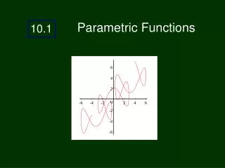
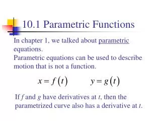
2. 10.1 Parametric Functions The formula for finding the slope of a parametrized curve is: This makes sense if we think about canceling dt.

3. 10.1 Parametric Functions The formula for finding the slope of a parametrized curve is: We assume that the denominator is not zero.

4. 10.1 Parametric Functions To find the second derivative of a parametrized curve, we find the derivative of the first derivative: • Find the first derivative (dy/dx). 2. Find the derivative of dy/dx with respect to t. 3. Divide by dx/dt.

5. 10.1 Parametric Functions

6. 10.1 Parametric Functions • Find the first derivative (dy/dx).

7. 10.1 Parametric Functions 2. Find the derivative of dy/dx with respect to t. Quotient Rule

8. 10.1 Parametric Functions 3. Divide by dx/dt.

9. 10.1 Parametric Functions The equation for the length of a parametrized curve is similar to our previous “length of curve” equation:

10. 10.1 Parametric Functions

11. 10.1 Parametric Functions This curve is:

12. 10.2 Vectors in the Plane Quantities that we measure that have magnitude but not direction are called scalars. Quantities such as force, displacement or velocity that have direction as well as magnitude are represented by directed line segments. B terminal point The length is initial point A

13. 10.2 Vectors in the Plane B terminal point A initial point A vector is represented by a directed line segment. Vectors are equal if they have the same length and direction (same slope).

14. 10.2 Vectors in the Plane y A vector is in standard position if the initial point is at the origin. x The component form of this vector is:

15. 10.2 Vectors in the Plane y A vector is in standard position if the initial point is at the origin. x The component form of this vector is: The magnitude (length) of is:

16. 10.2 Vectors in the Plane The component form of (-3,4) P is: (-5,2) Q v (-2,-2)

17. 10.2 Vectors in the Plane Then v is a unit vector. If is the zero vector and has no direction.

18. 10.2 Vectors in the Plane Vector Operations: (Add the components.) (Subtract the components.)

19. 10.2 Vectors in the Plane Vector Operations: Scalar Multiplication: Negative (opposite):

20. 10.2 Vectors in the Plane

21. 10.2 Vectors in the Plane

22. 10.2 Vectors in the Plane

23. 10.2 Vectors in the Plane u v u + v is the resultant vector. u+v (Parallelogram law of addition) v u

24. 10.2 Vectors in the Plane The angle between two vectors is given by: This comes from the law of cosines. See page 524 for the proof if you are interested.

25. 10.2 Vectors in the Plane The dot product (also called inner product) is defined as: Read “u dot v” This could be substituted in the formula for the angle between vectors to give:

26. 10.2 Vectors in the Plane

27. 10.2 Vectors in the Plane

28. 10.2 Vectors in the Plane Application: Example 7 A Boeing 727 airplane, flying due east at 500 mph in still air, encounters a 70-mph tail wind acting in the direction of 60o north of east. The airplane holds its compass heading due east but, because of the wind, acquires a new ground speed and direction. What are they?

29. 10.2 Vectors in the Plane N E u

30. 10.2 Vectors in the Plane N v 60o E u

31. 10.2 Vectors in the Plane N We need to find the magnitude and direction of the resultant vectoru + v. v u+v E u

32. 10.2 Vectors in the Plane N The component forms of u and v are: v 70 u+v E 500 u Therefore:

33. 10.2 Vectors in the Plane N 538.4 6.5o E The new ground speed of the airplane is about 538.4 mph, and its new direction is about 6.5o north of east.

34. 10.3 Vector-valued Functions Any vector can be written as a linear combination of two standard unit vectors. The vector v is a linear combination of the vectors i and j. The scalar a is the horizontal component of v and the scalar b is the vertical component of v.

35. 10.3 Vector-valued Functions If we separate r(t) into horizontal and vertical components, we can express r(t) as a linear combination of standard unit vectors i and j.

36. 10.3 Vector-valued Functions AB = <6,3> = 6i + 3j Let A = (-2,3) and B = (4,6) Find AB in terms of i and j

37. 10.3 Vector-valued Functions In three dimensions the component form becomes:

38. 10.3 Vector-valued Functions Most of the rules for the calculus of vectors are the same as we have used, except: “Absolute value” means “distance from the origin” so we must use the Pythagorean theorem.

39. 10.3 Vector-valued Functions b) Find the velocity, acceleration, speed and direction of motion at . a) Find the velocity and acceleration vectors.

40. 10.3 Vector-valued Functions b) Find the velocity, acceleration, speed and direction of motion at . velocity: acceleration:

41. 10.3 Vector-valued Functions b) Find the velocity, acceleration, speed and direction of motion at . speed: direction:

42. 10.3 Vector-valued Functions a) Write the equation of the tangent where . At : position: slope: tangent:

43. 10.3 Vector-valued Functions b) Find the coordinates of each point on the path where the horizontal component of the velocity is 0. The horizontal component of the velocity is .

44. 10.3 Vector-valued Functions a) Write the equation of the tangent where t = 1. r(t) = (2t2- 3t)i + (3t3- 2t)j v(t) = (4t - 3)i + (9t2 - 2)j v(1) = 1i + 7j At t = 1 r(1) = -1i + 1j position: slope: (-1,1) tangent:

45. 10.3 Vector-valued Functions b) Find the coordinates of each point on the path where the horizontal component of the velocity is 0. The horizontal component of the velocity is 4t - 3 . 4t – 3 = 0

46. 10.3 Vector-valued Functions Find r

47. 10.4 Projectile Motion One early use of calculus was to study projectile motion. In this section we assume ideal projectile motion: Constant force of gravity in a downward direction Flat surface No air resistance (usually)

48. 10.4 Projectile Motion We assume that the projectile is launched from the origin at time t=0 with initial velocity vo. The initial position is:

49. 10.4 Projectile Motion Newton’s second law of motion: Vertical acceleration

50. 10.4 Projectile Motion Newton’s second law of motion: The force of gravity is: Force is in the downward direction