Download
1 / 65
670 likes | 836 Vues
Performance Characteristics of Sensors and Actuators. (Chapter 2). Input and Output. Sensors Input: stimulus or measurand (temperature pressure, light intensity, etc.) Ouput: electrical signal (voltage, current frequency, phase, etc.)

E N D
Performance Characteristics of Sensors and Actuators (Chapter 2)
Input and Output • Sensors Input: stimulus or measurand (temperature pressure, light intensity, etc.) Ouput: electrical signal (voltage, current frequency, phase, etc.) Variations: output can sometimes be displacement (thermometers, magnetostrictive and piezoelectric sensors). Some sensors combine sensing and actuation
Input and Output • Actuators Input: electrical signal (voltage, current frequency, phase, etc.) Output: mechanical(force, pressure, displacement) or display function (dial indication, light, display, etc.)
Transfer function • Relation between input and output • Other names: • Input output characteristic function • transfer characteristic function • response
Transfer function (cont.) • Linear or nonlinear • Single valued or not • One dimensional or multi dimensional • Single input, single output • Multiple inputs, single output • In most cases: • Difficult to describe mathematically (given graphically) • Often must be defined from calibration data • Often only defined on a portion of the range of the device
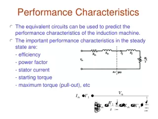
Transfer function (cont.) • T1 to T2 - approximately linear • Most useful range • Typically a small portion of the range • Often taken as linear
Transfer function (cont.) • Other data from transfer function • saturation • sensitivity • full scale range (input and output) • hysteresis • deadband • etc.
Transfer function (cont.) • Other types of transfer functions • Response with respect to a given quantity • Performance characteristics (reliability curves, etc.) • Viewed as the relation between any two characteristics
Impedance and impedance matching • Input impedance: ratio of the rated voltage and the resulting current through the input port of the device with the output port open (no load) • Output impedance: ratio of the rated output voltage and short circuit current of the port (i.e. current when the output is shorted) • These are definitions for two-port devices
Impedance (cont.) • Sensors: only output impedance is relevant • Actuators: only input impedance is relevant • Can also define mechanical impedance • Not needed - impedance is important for interfacing • Will only talk about electrical impedance
Impedance (cont.) • Why is it important? It affects performance • Example: 500 W sensor (output impedance) connected to a processor • b. Processor input impedance is infinite • c. Processor input impedance is 500 W
Impedance (cont.) • Example. Strain gauge: impedance is 500 W at zero strain, 750 W at measured strain • b: sensor output: 2.5V (at zero strain), 3V at measured strain • c. sensor output: 1.666V to 1.875V • Result: • Loading in case c. • Reduced sensitivity(smaller output change for the same strain input) • b. is better than c (in this case). Infinite impedance is best.
Impedance (cont.) • Current sensors: impedance is low - need low impedance at processor • Same considerations for actuators • Impedance matching: • Sometimes can be done directly (C-mos devices have very high input impedances) • Often need a matching circuit • From high to low or from low to high impedances
Impedance (cont.) • Impedance can (and often is) complex: Z=R+jX • In addition to the previous: • Conjugate matching (Zin=Zout*) - maximum power transfer • Critical for actuators! • Usually not important for sensors • Zin=R+jX, Zout*=R-jX. • No reflection matching (Zin=Zout) - no reflection from load • Important at high frequencies (transmission lines) • Equally important for sensors and actuators (antennas)
Range and Span • Range: lowest and highest values of the stimulus • Span:the arithmetic difference between the highest and lowest values of the stimulus that can be sensed within acceptable errors • Input full scale (IFS) = span • Output full scale (OFS): difference between the upper and lower ranges of the output of the sensor corresponding to the span of the sensor • Dynamic range:ratio between the upper and lower limits and is usually expressed in db
Range and Span (Cont) • Example: a sensors is designed for: -30 C to +80 C to output 2.5V to 1.2V • Range: -30C and +80 C • Span: 80- (-30)=110 C • Input full scale = 110 C • Output full scale = 2.5V-1.2V=1.3V • Dynamic range=20log(140/30)=13.38db
Range and Span (cont.) • Range, span, full scale and dynamic range may be applied to actuators in the same way • Span and full scale may also be given in db when the scale is large. • In actuators, there are other properties that come into play: • Maximum force, torque, displacement • Acceleration • Time response, delays, etc.
Accuracy, errors, repeatability • Errors: deviation from “ideal” • Sources: • materials used • construction tolerances • ageing • operational errors • calibration errors • matching (impedance) or loading errors • noise • many others
Accuracy, errors (cont.) • Errors: defined as follows: • a. As a difference: e = V – V0 (V0 is the actual value, V is that measured value (the stimulus in the case of sensors or output in actuators). • b. As a percentage of full scale (span for example) e = t/(tmax-tmin)*100 where tmax and tmin are the maximum and minimum values the device is designed to operate at. • c. In terms of the output signal expected.
Example: errors • Example: A thermistor is used to measure temperature between –30 and +80 C and produce an output voltage between 2.8V and 1.5V. Because of errors, the accuracy in sensing is ±0.5C.
Example (cont) • a. In terms of the input as ±0.5C • b. Percentage of input: e = 0.5/(80+30)*100 = 0.454% • c. In terms of output. From the transfer function: e= ±0.059V.
More on errors • Static errors: not time dependent • Dynamic errors: time dependent • Random errors: Different errors in a parameter or at different operating times • Systemic errors: errors are constant at all times and conditions
Error limits - linear TF • Linear transfer functions • Error equal along the transfer function • Error increases or decreases along TF • Error limits - two lines that delimit the output
Error limits - nonlinear TF • Nonlinear transfer functions • Error change along the transfer function • Maximum error from ideal • Average error • Limiting curves follow ideal transfer function
Error limits - nonlinear TF • Calibration curve may be used when available • Lower errors • Maximum error from calibration curve • Average error • Limiting curves follow the actual transfer function (calibration)
Repeatability • Also called reproducibility: failure of the sensor or actuator to represent the same value (i.e. stimulus or input) under identical conditions when measured at different times. • usually associated with calibration • viewed as an error. • given as the maximum difference between two readings taken at different times under identical input conditions. • error given as percentage of input full scale.
Sensitivity • Sensitivity of a sensor is defined as the change in output for a given change in input, usually a unit change in input. Sensitivity represents the slope of the transfer function. • Same for actuators
Sensitivity • Sensitivity of a sensor is defined as the change in output for a given change in input, usually a unit change in input. Sensitivity represents the slope of the transfer function. • Same for actuators
Sensitivity (cont.) • Example for a linear transfer function: • Note the units • a is the slope • For the transfer function in (2):
Sensitivity (cont.) • Usually associated with sensors • Applies equally well to actuators • Can be highly nonlinear along the transfer function • Measured in units of output quantity per units of input quantity (W/C, N/V, V/C, etc.)
Sensitivity analysis (cont.) • A difficult task • there is noise • a combined function of sensitivities of various components, including that of the transduction sections. • device may be rather complex with multiple transduction steps, each one with its own sensitivity, sources of noise and other parameters • some properties may be known but many may not be known or may only be approximate. Applies equally well to actuators
Sensitivity analysis (cont.) • An important task • provides information on the output range of signals one can expect, • provides information on the noise and errors to expect. • may provide clues as to how the effects of noise and errors may be minimized • Provides clues on the proper choice of sensors, their connections and other steps that may be taken to improve performance (amplifiers, feedback, etc.).
Example - additive errors • Fiber optic pressure sensor • Pressure changes the length of the fiber • This changes the phase of the output • Three transduction steps
Example-1 - no errors present • Individual sensitivities • Overall sensitivity • But, x2=y1 (output of transducer 1 is the input to transducer 2) and x3=y2
Example -1 - errors present • First output is y1=y01 + y1. y01 = Output without error • 2nd output • 3rd output Last 3 terms - additive errors
Example -2 - differential sensors • Output proportional to difference between the outputs of the sensors • Output is zero when T1=T2 • Common mode signals cancel (noise) • Errors cancel (mostly)
Example -3 - sensors in series • Output is in series • Input in parallel (all sensors at same temperature) • Outputs add up • Noise multiplied by product of sensitivities
Hysteresis • Hysteresis (literally lag)- the deviation of the sensor’s output at any given point when approached from two different directions • Caused by electrical or mechanical systems • Magnetization • Thermal properties • Loose linkages
Hysteresis - Example • If temperature is measured, at a rated temperature of 50C, the output might be 4.95V when temperature increases but 5.05V when temperature decreases. • This is an error of ±0.5% (for an output full scale of 10V in this idealized example). • Hysteresis is also present in actuators and, in the case of motion, more common than in sensors.
Nonlinearity • A property of the sensor (nonlinear transfer function) or: • Introduced by errors • Nonlinearity errors influence accuracy. • Nonlinearity is defined as the maximum deviation from the ideal linear transfer function. • The latter is not usually known or useful • Nonlinearity must be deduced from the actual transfer function or from the calibration curve • A few methods to do so:
Nonlinearity (cont.) • a. by use of the range of the sensor/actuator • Pass a straight line between the range points (line 1) • Calculate the maximum deviation of the actual curve from this straight line • Good when linearities are small and the span is small (thermocouples, thermistors, etc.) • Gives an overall figure for nonlinearity
Nonlinearity (cont.) • b. by use of two points defining a portion of the span of the sensor/actuator. • Pass a straight line between the two points • Extend the straight line to cover the whole span • Calculate the maximum deviation of the actual curve from this straight line • Good when a device is used in a small part of its span (i.e. a thermometer used to measure human body temperatures • Improves linearity figure in the range of interest
Nonlinearity (cont.) • c. use a linear best fit(least squares) through the points of the curve • Take n points on the actual curve, xi,yi, i=1,2,…n. • Assume the best fit is a line y=ax+b (line 2) • Calculate a and b from the following:
Nonlinearity (cont.) • d. use the tangent to the curve at some point on the curve • Take a point in the middle of the range of interest • Draw the tangent and extend to the range of the curve (line 3) • Calculate the nonlinearity as previously • Only useful if nonlinearity is small and the span used very small
Saturation • Saturation a property of sensors or actuators when they no longer respond to the input. • Usually at or near the ends of their span and indicates that the output is no longer a function of the input or, more likely is a very nonlinear function of the input. • Should be avoided - sensitivity is small or nonexistent • In actuators, it can lead to failure of the actuator (increase in power loss, etc.)
Frequency response • Frequency response: The ability of the device to respond to a harmonic (sinusoidal) input • A plot of magnitude (power, displacement, etc.) as a function of frequency • Indicates the range of the stimulus in which the device is usable (sensors and actuators) • Provides important design parameters • Sometimes the phase is also given (the pair of plots is the Bode diagram of the device)
Frequency response (cont) • Important design parameters • Bandwidth (B-A, in Hz) • Flat frequency range (D-C in Hz) • Cutoff frequencies (points A and B in Hz) • Resonant frequencies
Frequency response (cont.) • Bandwidth: the distance in Hz between the half power points • Half-power points: eh=0.707e, ph=0.5p • Flat response range: maximum distance in Hz over which the response is flat (based on some allowable error) • Resonant frequency: the frequency (or frequencies) at which the curve peaks or dips