Exploring Matrix Algorithms in MATLAB: Power Method, Subspace Iteration, and QR Algorithm
This guide provides an introduction to key matrix algorithms implemented in MATLAB, focusing on the Power Method, Subspace Iteration, and the QR Algorithm. You'll find essential M-script files such as PowerMethod.m and ShowPowerMethod.m tailored for experimentation. Start MATLAB and explore how diagonal and orthogonal matrices are constructed. Learn through interactive demonstrations, tracking convergence, and adjusting shift parameters to observe algorithm performance. Ideal for students and researchers in numerical linear algebra.

Exploring Matrix Algorithms in MATLAB: Power Method, Subspace Iteration, and QR Algorithm
E N D
Presentation Transcript
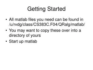
Getting Started • All matlab files you need can be found in /u/rvdg/class/CS383C.F04/QRalg/matlab/ • You may want to copy these over into a directory of yours • Start up matlab
The Power Method • The first demonstration centers around the Power Method • Two M-script files are involved: • PowerMethod.m • This is the main driver • ShowPowerMethod.m • This is a utility routine that prints out interesting stuff
Enter matrix size A random diagonal matrix is created Hit “Return” A random orthogonal matrix is created A random matrix is created Hit “Return”
Keep an eye on this The first element should become 1 (since q should eventually be the direction of the first column of U). The other elements should become 0 (since q should eventually be orthogonal To the other columns of U.) Current estimate of lambda(1) Actual lambda(1) Hit “Return”
Here I report the ratios | lj|/|l1| as the i-th element of this vector Notice that the component of q in the direction of uj should decrease in every iteration by a factor roughly equal to | lj|/|l1| Notice that the jth component of UT * q equals the length of the component of q in the direction of uj. By looking at this ratio, we are tracking by what factor these components are decreasing in each step.
I hit return a few times !!!!! Starting to look like we want!
I hit return a few more times !!!!! Starting to look like we want!
Finally reply “0” (or anything else but a return)
Subspace Iteration • The second demonstration centers around the relation between the Power Method and Subspace Iteration
Hit “return” a few times to create a random matrix, etc.
The Power Method and Subspace Iteration are now both tracked
A few iterations later Again, these are the factors by which we would predict that components in the directions of uj would decrease (see similar discussion for power method.)
QR algorithm • The third demonstration centers around the relation between Subspace Iteration and the QR algorithm
Recall the QR algorithm: A0 = A For i=0,… Ai – r I = QR Ai+1 = R Q + r I
The difference here simply comes from a different number of digits being printed
For now, just use shift rho = 0 by hitting return every time
A few more iterations later… All off-diagonal elements are starting to become small
QR algorithm • The fourth demonstration centers around the effects of choosing shifts
Notice MUCH faster convergence to zero!
A few iterations later… A few iterations later…
Now these elements are converging faster