Understanding ANOVA: A Comprehensive Guide to Testing Population Means
250 likes | 660 Vues
Analysis of Variance (ANOVA) is a statistical method used to determine if there are significant differences among three or more population means. By testing the null hypothesis (H0: μ1 = μ2 = ... = μk), ANOVA assesses whether at least two means are different. Key assumptions include normal distribution of data, equal variances across populations, and independence of observations. The F-test is applied to compare variances, and if significant differences are found, post-hoc tests like Fisher’s LSD can identify where those differences lie. This guide provides insights into conducting ANOVA and interpreting results effectively.

Understanding ANOVA: A Comprehensive Guide to Testing Population Means
E N D
Presentation Transcript
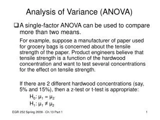
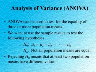
Analysis of Variance (ANOVA) • ANOVA can be used to test for the equality of three or more population means • We want to use the sample results to test the following hypotheses. H0: 1=2=3=. . . = k Ha: Not all population means are equal • Rejecting H0 means that at least two population means have different values.
Assumptions of ANOVA • The values from each population are normally distributed. • The variance, 2, is the same for all of the populations. • The observations must be independent.
Impact of Assumptions • Given these assumptions, what is the source of variation among the observed variables? Two values could come from different populations, or distributions, which could have different means. Two values could come from the same distribution.
ANOVA:Testing for the Equality of k Population Means • The ANOVA table • Between-treatments estimate of 2 • Within-treatments estimate of 2 • Comparing these two estimates: The F Test
Preliminaries • Compute the jth sample mean and variance, j = 1,…,k • Compute the overall sample mean Note: the book calls this nT
Between-Treatment Estimate of 2 • Sum of squares due to treatments • A between-treatments estimate of 2, MSTR, can be computed by
Within-Treatment Estimate of 2 • The within-treatments estimate of 2
The ANOVA Table Source of Sum of Degrees of Mean Variation Squares Freedom Squares F Between SSTR k - 1 MSTR MSTR/MSE Within SSE nT - k MSE Total SST nT - 1
Example: Kelli Home Products, Inc. • Kelli Home Products, Inc. is considering marketing a long lasting car wax. Three different waxes (Type 1, Type 2, and Type 3) have been developed. In order to test the durability of these waxes, 5 new cars were waxed with Type 1, 5 with Type 2, and 5 with Type 3. Each car was then repeatedly run through an automatic carwash until the wax coating showed signs of deterioration. The number of times each car went through the carwash is shown on the next slide. Kelli Home Products, Inc. must decide which wax to market. Are the three waxes equally effective?
Example continued ObservationType 1Type 2Type 3 1 48 73 51 2 54 63 63 3 57 66 61 4 54 64 54 5 62 74 56 Sample Mean 55 68 57 Sample Variance 26.0 26.5 24.5
The F-Test • If the null hypothesis is true and the ANOVA assumptions are valid, the sampling distribution of MSTR/MSE is an F distribution with k – 1 numerator and nT – k denominator df • If the means of the k populations are not equal, the value of MSTR/MSE will be inflated because MSTR overestimates 2.
Reject H0 MSTR/MSE F Critical Value Sampling Distribution of MSTR/MSE • The figure below shows the rejection region associated with a level of significance equal to where F denotes the critical value. Do Not Reject H0
The F-Test • We will reject H0 if the resulting value of MSTR/MSE appears to be too large to have been selected at random from the appropriate F distribution. • Our decision rule becomes
Example continued • Assuming = .05, F.05 = 3.89 (2 d.f. numerator, 12 d.f. denominator). Therefore, reject H0 if F > 3.89 • Test Statistic: F = MSTR/MSE = 245/25.667 = 9.55 • Decision: Reject H0 • There appears to be a difference in the types of wax at a 5% level of significance.
Multiple Comparison Procedures • If ANOVA provides statistical evidence to reject the null hypothesis of equal population means, then Fisher’s least significance difference (LSD) procedure can be used to determine where the differences occur.
Fisher’s LSD Procedure • Pairwise hypothesis tests of the form • Test Statistic
Fisher’s LSD Procedure • Rejection rule:
Alternative Fisher’s LSD Procedure • Hypotheses • Rejection Rule where
Using LSD in our Example • Assuming = .05, t.025,12 = 2.179. • Test Statistic • Conclusion The mean number of hours worked at Plant 1 is not equal to the mean number worked at Plant 2.
Using LSD in our Example • Note that • Since 13 > 6.98, and 11 > 6.98, we conclude that types 1 and 2 have different means, and types 2 and 3 have different means, but there is no significant difference between the means of types 1 and 3.
Getting it Done in EXCEL • Use Tools/Data Analysis/ANOVA: Single Factor • Data should be in columns which represent each treatment
Experimental Design • Statistical studies can be classified as being either experimental or observational. • In an experimental study, one or more factors are controlled so that data can be obtained about how the factors influence the variables of interest. • In an observational study, no attempt is made to control the factors. • Cause-and-effect relationships are easier to establish in experimental studies than in observational studies.